Exporting data to Excel often results in empty rows scattering throughout the worksheet. As manually deleting each blank row is a tedious task, we’ll show you all the different ways to delete all empty rows at once.
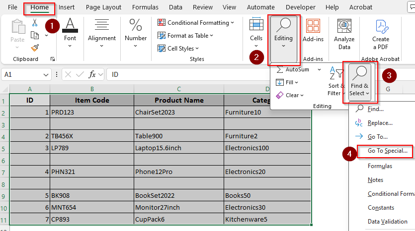
➤ To delete blank rows, select your data range and go to the Home tab. Click on Editing >> Find & Select >> Go To Special.
➤ Or, press the keyboard shortcuts CTRL + G and click on Special.
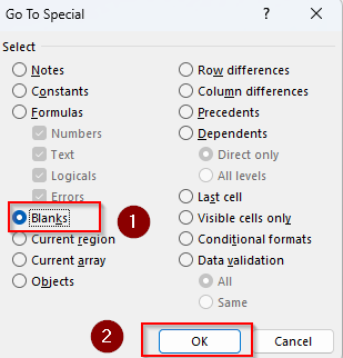
➤ From the Go To Special box, select Blanks and click Ok.
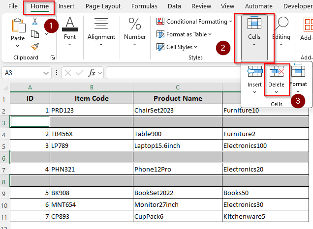
➤ As Excel highlights the empty rows, you need to go to the Home tab, click on Cells, and choose Delete.
However, this method doesn’t protect rows that have only one or two empty cells. From this article, you’ll learn how to delete empty rows and protect rows with blank cells using various filters, functions, Power Query, etc.
Manually Deleting Cells with the Delete Option
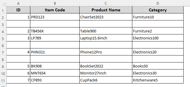
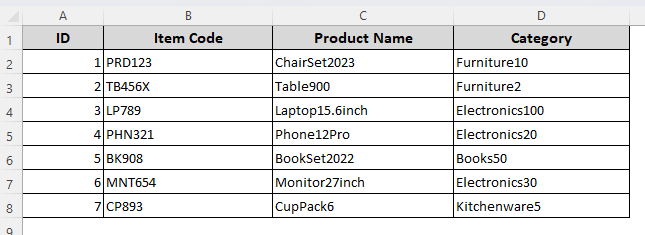
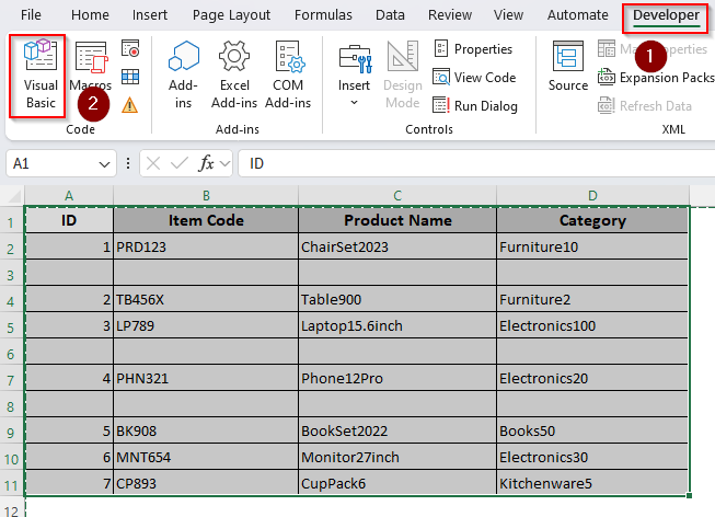
In our dataset, we entered some product data for a store. As you can see, rows number 3, 6, and 8 are completely empty. Our task is to delete these rows to organize our data better.
If your data set only contains a few empty rows that you can easily locate, you can delete each row manually. Follow the steps given below:
➤ Press the CTRL key on your keyboard and click on the row numbers representing each row you want to delete.
➤ Make sure you press and hold the CTRL button to highlight all these rows at once.
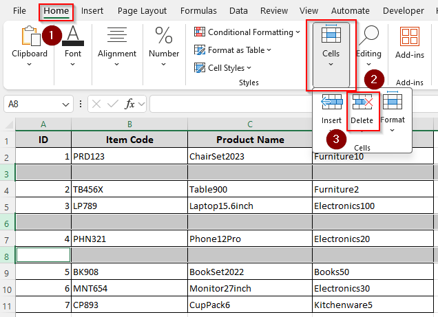
➤ Once you’re done highlighting the rows, go to the Home tab and select the Cells option. Choose Delete from the menu.
➤ Now all the empty rows you selected are deleted and the data should be sorted like this:
Deleting Empty Rows with the Find & Select Tool
With this method, you can delete completely empty rows as well as rows with blank cells. Excel will delete the entire row even if other cells of the row contain some data. So, avoid it if you want to protect the cells with data.
To remove all the rows with empty cells, follow these steps:
➤ Select your entire data range and click on the Editing option from the Home tab.
➤ Choose Find & Select from the Editing group and click on Go To Special from the drop-down menu.

➤ Another way to go to the special options is by using the keyboard shortcuts CTRL + G and selecting Special.
➤ As the Go To Special box arrives, you need to select Blanks from the options and click Ok.
➤ Now, Excel will highlight all the blank cells from your selected data range. From the Home tab, click on Cells, and choose Delete.
Sort Out Empty Rows and Delete
Use this method if you don’t get bothered rearranging your data in an ascending/descending alphabetical or numerical order. As you apply the sorting tool, Excel pushes all the empty rows of your sheet to the bottom of your data range.
Therefore, you can easily select and remove them at once. Here’s how to do it:
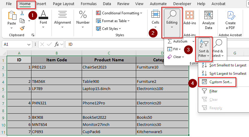
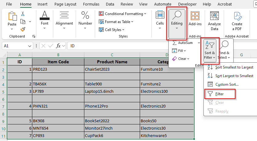
➤ Select your data range and go to the Home tab. Click on Editing and select Sort & Filter.
➤ From the drop-down menu, choose Custom Sort.
➤ As the Sort box arrives, click on the arrow beside the Sort By box under the Column title.
➤ Our data has a numerical column which is the ID column. So, we picked this column from the drop-down menu.
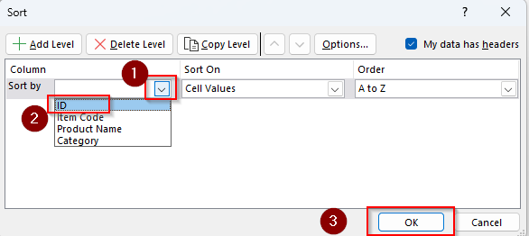
➤ You can choose any column you prefer if you don’t have numerically sorted data. In this case, the sorting will be done alphabetically.
➤ Click Ok and Excel will sort the empty rows at the bottom.
➤ Select all the blank rows and press Delete from the Cells group.

Apply a Filter to Eliminate Empty Rows
When you want to protect rows that contain some blank cells and a few non-blank cells, you can protect such cells with this method. Here, we’ll filter out the blank rows first and delete them manually. Let’s get to the process:
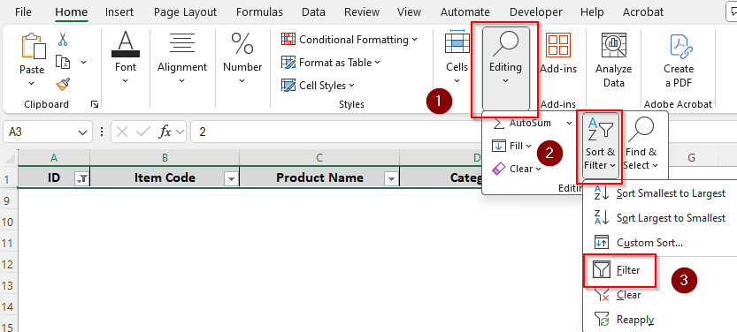
➤ Select your data range and press CTRL + SHIFT + L to apply a filter.
➤ Or, you can click on the Sort & Filter tool from the Editing group.
➤ Choose Filter from the drop-down menu.
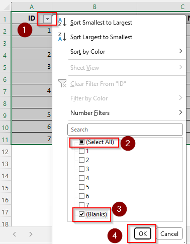
➤ Go to the first column and click on the small downward arrow sign in the header cell.
➤ From the drop-down menu, uncheck Select All.
➤ Scroll down and check the Blanks box. Press Ok, and only the blank cells will appear on the screen.
➤ Now, if you have non-blank cells, Excel will display the values from those cells. In this case, you need to repeat the previous steps for all the columns of your data.
➤ Once all the rows are completely empty, select the rows without the header row. Click on Delete from the Cells group.
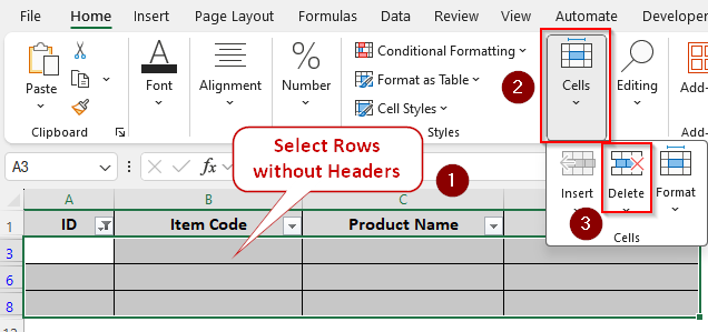
➤ Excel will send you a warning asking if you want to delete the entire sheet row. Click Ok and the empty rows are now removed.
![]()
➤ To get back your data, go back to Sort & Filter and click on Filter to clear the filter off.
Applying the COUNTA Function and a Filter
Similar to the previous method, using the COUNTA function and applying a filter will protect rows with combined blank and non-blank cells. For every blank row, the COUNTA function gives a zero.
So, our task is to filter out and delete all the cells with the value 0. Here are the steps:
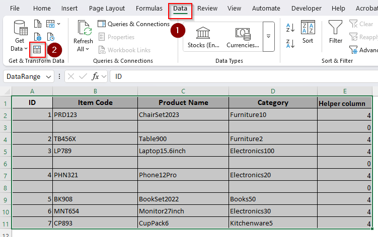
➤ Create a helper column and type the following formula for your first data row:
=COUNTA(A2:D2)
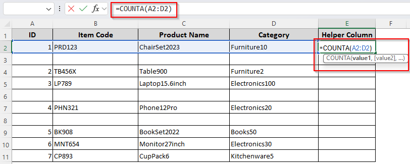
➤ Replace the cell range (A2:D2) with the specific range of your row. You can also select them using your cursor.
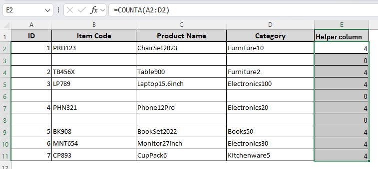
➤ Press Enter and Excel will count how many occupied cells are there in the chosen row.
➤ Drag the formula until the last row of your data range using the tiny black + sign on the lower corner of the cell.
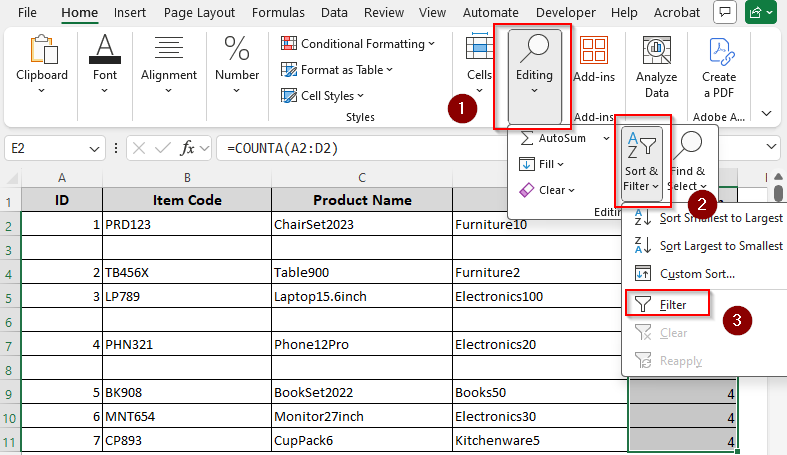
➤ Now, select the helper cell and click on Editing and choose Sort & Filter. Choose Filter from the menu.
➤ Click on the downward arrow from the first cell and uncheck the Select All box from the new menu.
➤ Check the 0 box and click Ok.
![]()
➤ At this point, Excel will display the cells with the value zero. Select all these cells from the helper column and click Delete from the Cells group.
![]()
➤ Excel has now deleted all the empty cells from your worksheet. You can keep the helper column or delete it.
➤ To remove the column, select the entire column and press Delete.
![]()
Using the Power Query Tool
For lengthy and complex datasets, using the Power Query tool is the best solution. As it’s a dynamic tool, you can utilize it to prevent creating empty rows in the future. Let’s learn how to use it:
➤ Start by selecting your entire data range. If you want to add more data later, you can select some extra rows or simply press CTRL + A to select the entire sheet.
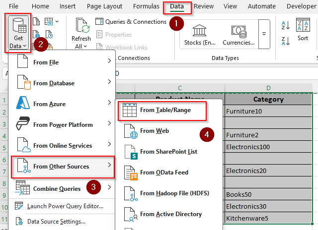
➤ Go to the Data tab and click on Get Data from the Get & Transform Data group.
➤ As a drop-down menu appears, choose From Other Sources and then select From Table/Range.
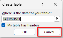
➤ Now, Excel will display a Create Table box so that it can convert your selected data range into a table. However, our data isn’t in a table, so we click on Cancel.
➤ Instead of creating a table, we will go to the Name Box and type a name for our data range. You can select any name you want, but make sure the name doesn’t have any space.
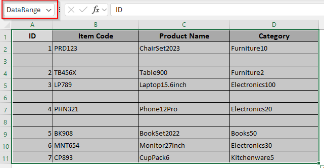
➤ Press Enter and go to the Data tab. Click on the From Table/Range icon.
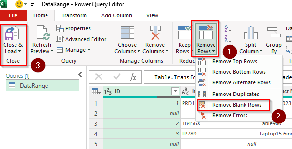
➤ As the Power Query Editor opens, select Remove Rows and then choose Remove Blank Rows.
➤ Click on Close & Load and Excel will remove the blank rows.
➤ When you use the Power Query tool, it changes the layout of your sheet. To change it, go to the Table Design tab and select any of your preferred Table Styles.
![]()
Applying a VBA Macro
With Microsoft’s Visual Basic, you can create a code to delete completely empty rows. Here’s the process:
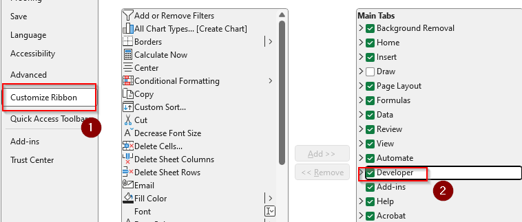
➤ To get the Developer tab on the main ribbon, go to File and select More. Choose Options from the menu.
➤ Click on Customize Ribbon and check Developer from the options. Press Ok.
➤ Select your data range, go to the Developer tab, and click on Visual Basic. You can also press ALT + F11 .
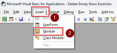
➤ In the VBA Editor press the Insert tab and choose Module from the menu.
➤ Paste the following code:
Sub DeleteEmptyRowsInSelection()
Dim selectedRange As Range
Dim rowRange As Range
Dim i As Long
Dim isEmpty As Boolean
' Set the selected range
On Error Resume Next
Set selectedRange = Selection
On Error GoTo 0
If selectedRange Is Nothing Then
MsgBox "Please select a range first.", vbExclamation
Exit Sub
End If
' Loop from the bottom row up to avoid skipping rows after deletion
For i = selectedRange.Rows.Count To 1 Step -1
Set rowRange = selectedRange.Rows(i)
isEmpty = Application.WorksheetFunction.CountA(rowRange) = 0
If isEmpty Then
rowRange.EntireRow.Delete
End If
Next i
MsgBox "Empty rows deleted.", vbInformation
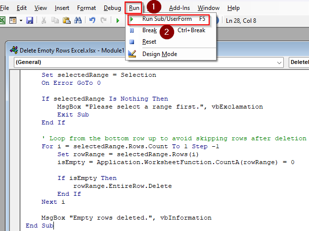
End Sub➤ From the top ribbon, select Run and click on Run Sub/UserForm.
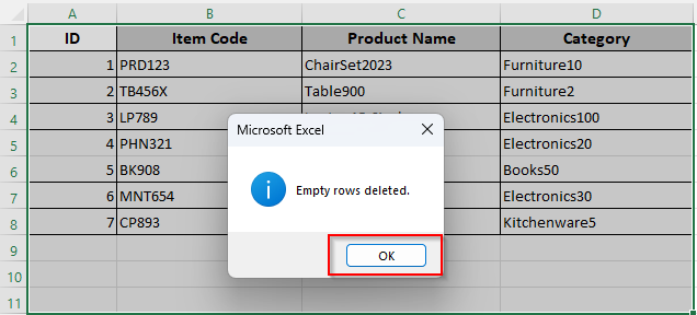
➤ At this point, Excel will sort your data without the empty rows and send a notification on your screen. Click Ok.
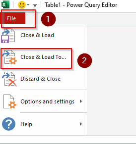
➤ To save the changes, go to Save As and navigate through your desired location.
➤ While saving the file make sure to choose Excel Macro-Enabled Workbook from the options for the Save As Type. Finally, click Save.
![]()
Frequently Asked Questions
How to remove blank cells from a row and extract data in Excel?
To remove blank cells and extract data from the occupied cells of that row, choose a different cell range in the worksheet to input the extracted data. Now, type the following formula:
=FILTER(A1:D1, NOT(ISBLANK(A1:D1)))
Replace A1:D1 with the cell references of your selected row. The formula filters the cells that are not blank in your selected location.
How do I delete empty infinite rows in Excel?
Identify the first blank row of your dataset and press SHIFT + SPACEBAR to select the row. Use the keyboard shortcut CTRL + SHIFT + DOWN ARROW to get to the end row of your sheet. From the Home tab, go to Cells and click on Delete.
How do you fill in blank cells with the value above?
Select your data range and click on the Home tab >> Find & Select >> Go To Special. Select blanks and click Ok. Type = in any of the highlighted cells and enter the cell reference from which you want to export data to your highlighted cell. For example, select the C3 cell and type:
=B3
Now, press CTRL + ENTER on your keyboard to repeat the process for all the highlighted blank cells.
Concluding Words
Depending on the number of rows you want to delete, some of the above-mentioned methods work better than others. For less complex datasets, sorting and using the Find & Select tool are two simple choices.
However, we recommend using Power Query when you’re dealing with hundreds of rows and columns. It’s also useful to prevent any occurrences of empty cells in your selected range.