
Rounding up a number to your preferred decimal points allows you to keep your dataset neat and easy to apply the results in real-life situations. Be it employee scheduling, shipping or packaging, counting raw materials, or invoicing, Excel gives you a dedicated ROUNDUP formula for this, alongside ROUND, MROUND, EVEN and ODD, and a formatting route that changes what you see without changing the stored value. This guide covers all six ways to round up a formula result in Excel.
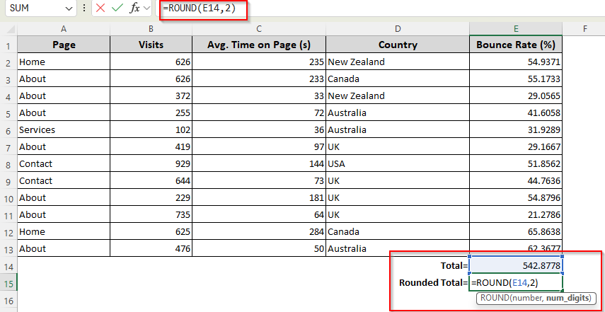
➤ To always round up the result of a formula, select a helper cell and enter:
=ROUNDUP(E14,2)
➤ Use =ROUND(E14,2) instead when you want normal rounding, where values below the halfway point round down.
➤ Replace E14 with the cell reference of your formula result. Instead of 2, you can enter the number of digits to which you want to round the given number after the decimal point.
➤ Press Enter and drag the formula along the column if you want to round more numbers in other cells.
Excel has more functions like ROUNDUP, ROUNDDOWN, EVEN, ODD, MROUND, etc., to round up a decimal number resulting from a formula. We have covered several different ways of rounding up a number in Excel.
Overview of Different Rounding Functions in Excel
To use the roundup-related functions perfectly, you must learn how to input the arguments correctly. The common syntax format for the roundup formulas is as follows:
=ROUND(number, num_digits)
Here, the number refers to the decimal number you want to round up. With num_digits, you specify how many numbers you want to keep after the decimal point. Let’s take a look at some examples for better understanding:
- If you set num_digit = 1, it rounds the number to one decimal place.
Example:
=ROUND(542.8778, 1) becomes 542.9
- If you set num_digit = 2, it rounds the number to two decimal places.
Example:
=ROUND(542.8778, 2) becomes 542.88
- If you set num_digit = 3, the number rounds to three decimal places.
Example:
=ROUND(542.8778, 3) becomes 542.878
- If you set num_digit=0, the number rounds to the nearest whole number (integer) and eliminates the fractions completely.
Example:
=ROUND(542.8778, 0) becomes 543
Rounding to fewer decimal places is also how you change significant figures in a result. We can also round up the numbers on the left side of the decimal point using negative digits. Here’s how:
- If you set num_digit = -1, the number rounds to the nearest multiple of 10.
Example:
=ROUND(542.8778, -1) becomes 540
- If you set num_digit = -2, the number rounds to the nearest multiple of 100.
Example:
=ROUND(542.8778, -2) becomes 500
- If you set num_digit = -3, the number rounds to the nearest multiple of 1000.
Example:
=ROUND(542.8778, -3) becomes 1000 (542.8778 is closer to 1000 than to 0, so it rounds up to the nearest multiple of 1000)
Although we used the ROUND function, you can use the same format for any roundup-related format with the num_digit argument. The same argument controls the result when you round percentages, since Excel stores a percentage as a decimal.
Format Cells to Round Up a Formula Result
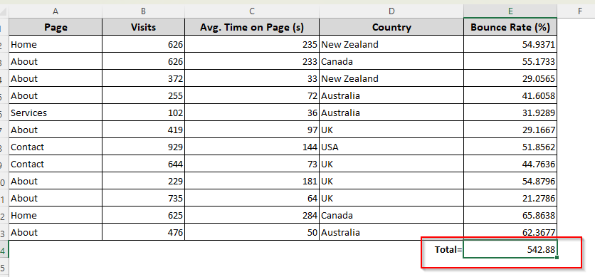
In our chosen dataset, we’re displaying the different elements of a website. For our roundup methods, we’ll use the Bounce Rate(%) column. We used the SUM function to add the numbers of this column.
While describing the methods, we will use the result of the SUM function to show you how to round the formula result to two places after the decimal point.
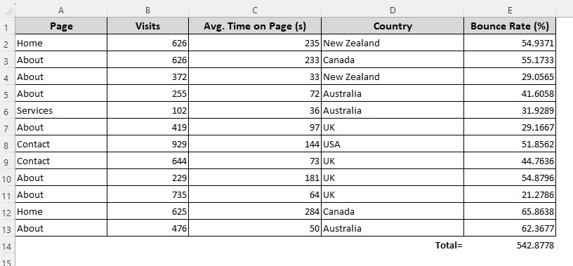
With this method, you can change the way a decimal number appears on the worksheet instead of actually changing it permanently. If you use the result in a different formula later, Excel will use the actual value instead of what is displayed on your screen. It is the quickest way to round numbers without a formula.
So, use it only when you want to protect the original value of a cell while making it look more neat. It is also the first thing to check when you want to stop Excel from rounding up decimals that you need to keep in full. Here are the steps:
➤ Click on the formula cell and go to the Home tab. Under the Number box, click on the Decrease Decimals sign to reduce decimals from the result.
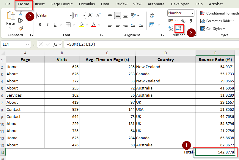
➤ If you want more customization, click on the arrow sign in the corner to launch the Format Cells dialog box. You can also launch it by pressing CTRL + 1 .
➤ On the Number tab, choose the right category according to your data type.
➤ In the Decimal Places box, type the numbers for how many digits of decimal places you want to keep in the result.
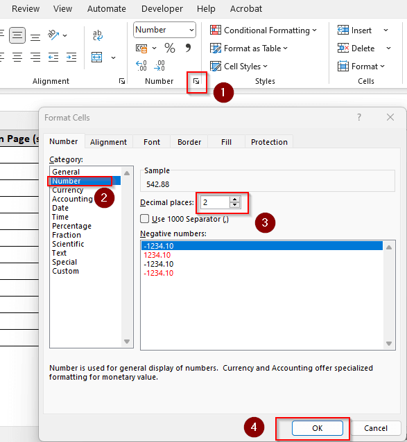
➤ Click Ok and Excel will change your data accordingly. Here’s the result for our dataset:
Using the ROUND Function
As the function rounds to the nearest number based on the traditional rounding rules, you can use the ROUND function for academic or financial work where you need mathematically accurate results.
It looks at the first digit being dropped: if that digit is 5 or greater the last kept digit moves up, and if it is less than 5 the last kept digit stays. Excel rounds halves away from zero, so =ROUND(2.5, 0) returns 3 and =ROUND(-2.5, 0) returns -3. Let’s apply it to our dataset.
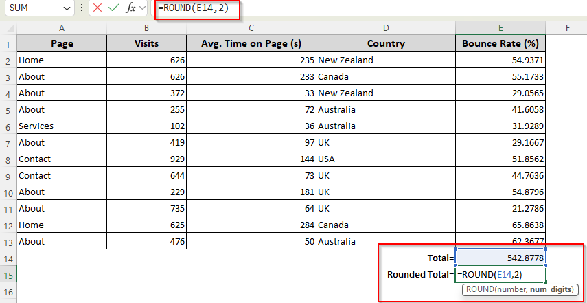
➤ Select the cell where you want to put the rounded number and type the following formula:
= ROUND(E14, 2)
➤ Replace E14 with the cell reference where you want the rounded result. Instead of 2, put the number of places you want to keep after the decimal point.
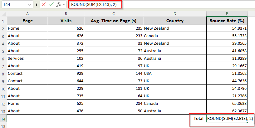
➤ If you prefer to integrate the ROUND function with the formula in a single cell, follow this format instead:
= ROUND(Formula, 2)
➤ Replace the Formula part with the correct formula you’ve used, and change the number of places after the decimal point as needed.
➤ You can also put the formula result directly like this:
= ROUND(542.8778, 2)
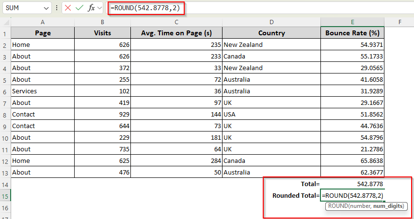
➤ Finally, press Enter. In all three cases, the result is as follows:
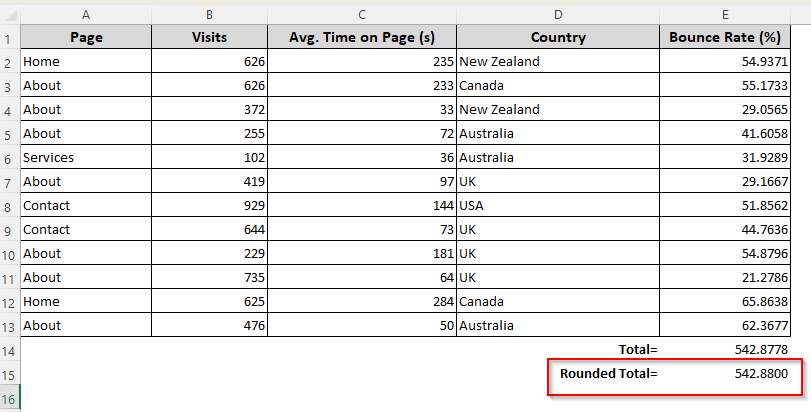
Applying the ROUNDUP or ROUNDDOWN Function
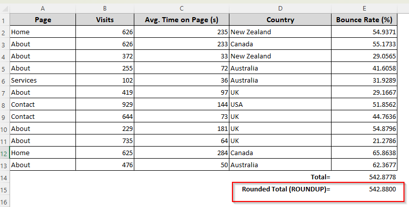
With the ROUNDUP function, you’ll always round a number up, away from zero. No matter how small the decimal part is, it will increase the preceding digit.
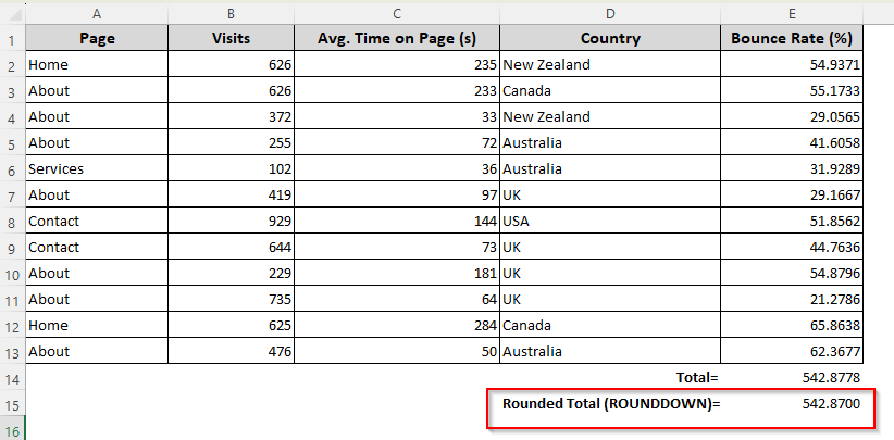
On the other hand, the ROUNDDOWN function always rounds a number down, towards zero. No matter how large the decimal part is, it truncates towards zero. For positive numbers that means a smaller result, and for negative numbers it means a result closer to zero: =ROUNDDOWN(-2.9, 0) returns -2, not -3. Set the second argument to 0 when you want to round down to the nearest whole number. Here’s how to use them:
➤ Select a cell to put the rounded result and type any of the following formulas and press Enter:
=ROUNDUP(E14, 2)
Or,
=ROUNDDOWN(E14, 2)
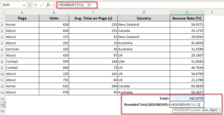
➤ Change the values E14 and 2 according to your required cell reference and the number of digits to which you want to round. You can also use the exact formula result or the formula itself instead of E14.
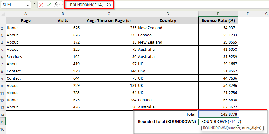
➤ The ROUNDUP function gives a value that is equal to or greater than the original number just like the picture given below:
➤ As for the ROUNDDOWN function, it gives a value that is equal to or less than the original number as shown in the picture below:
Rounding Up Numbers with the EVEN or ODD Function
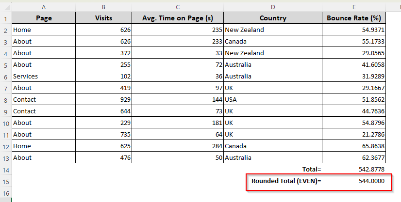
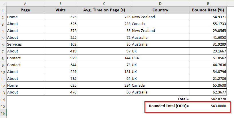
To round a number to the nearest even or odd integer while eliminating the fraction part, we use the EVEN and ODD functions in Excel. The EVEN function rounds away from zero to the nearest even integer and the ODD function rounds away from zero to the nearest odd integer. Both always move the number, so =ODD(2) returns 3 rather than leaving 2 unchanged, and =EVEN(-1.5) returns -2. Apply these functions using the following steps:
➤ Choose a cell to put the rounded number and type any of the following formulas:
=EVEN(E14)
Or,
=ODD(E14)
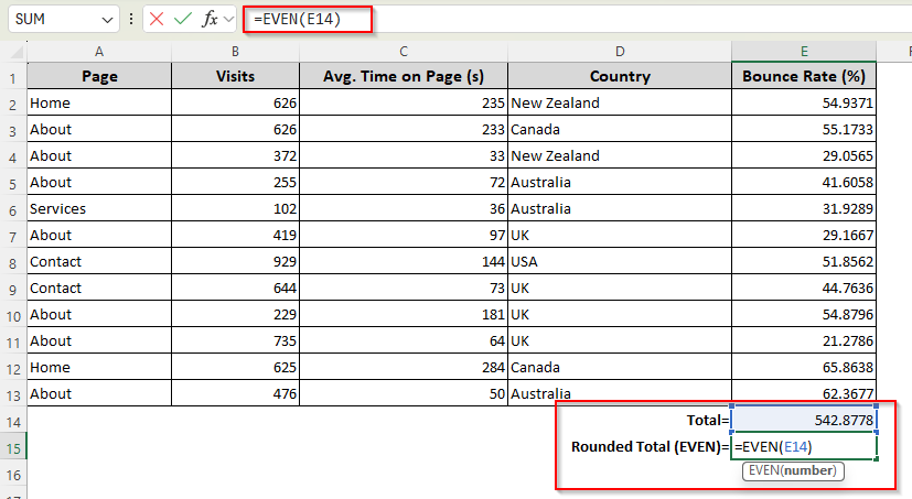
➤ Replace E14 with your chosen cell reference or the exact formula result you want to round up.
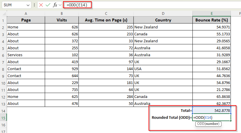
➤ Press Enter and the result for the EVEN function will look like this:
➤ Whereas, for the ODD function, you’ll get results similar to this:
Round Number to Specified Multiples with the MROUND Function
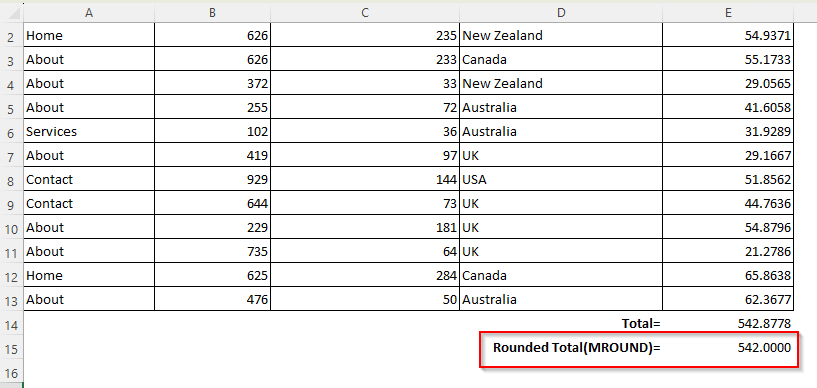
The MROUND function can round a formula result to the nearest multiple of your specified digit. It’s often used to round up currency, time, and other standard measuring units, which makes it the usual choice when you need to round time to the nearest 15 minutes. Here’s how to apply it:
➤ Click on a cell where you want to apply the formula and type the following:
=MROUND(E14, 2)

➤ Put your chosen cell value instead of E14. Replace 2 with the multiple to which you want to round the number. You can also apply a formula or its result directly.
➤ Press Enter and you’ll get the converted number rounded to the nearest multiple of your chosen digit.
Note:
MROUND returns a #NUM! error when the number and the multiple have different signs. For example, =MROUND(5, -2) returns #NUM! because 5 is positive and -2 is negative. Keep both arguments on the same side of zero. Also, there are the CEILING and FLOOR functions that work similarly. CEILING rounds away from zero to the nearest multiple of a specified digit, and FLOOR rounds towards zero. With negative numbers the modern CEILING.MATH and FLOOR.MATH functions give you an explicit mode argument, so reach for those when signs are mixed. Whereas, MROUND rounds up or down depending on which multiple is closer. One more limit worth knowing: when the multiple is a decimal, Microsoft documents the rounding direction at exact midpoints as undefined. =MROUND(6.05, 0.1) returns 6.0 while =MROUND(7.05, 0.1) returns 7.1, so do not rely on midpoint behaviour with decimal multiples.
Downloadable Resources
Get our practice workbook or necessary files that we have worked with to prepare this article.
Frequently Asked Questions
How do I add a round formula to multiple cells in Excel?
First, type the formula in the first cell of the column or row. Press Enter and drag the formula using the tiny black arrow sign in the bottom corner of the cell. Drag it until you cover all the cells you want to apply a round formula and release the cursor when you’re done.
How do you round a formula to a whole number?
To round a formula to a whole number and remove the fractions completely, type the following formula in your preferred cell:
=INT(542.8778)
In this case, the function will return 542. You can replace the number with a formula or cell reference.
Can you round a negative number in Excel?
Yes, you can round a negative number in Excel using functions like ROUNDUP, ROUND, and ROUNDDOWN. Let’s apply the ROUNDUP function for example. Select a cell and type:
=ROUNDUP(-542.8778, 2)
Excel will round up the result to two decimal places, resulting in -542.88.
Wrapping Up
With all the different formulas we’ve covered, you can easily round up a formula result in just a few clicks. Moreover, you can integrate each function with your original formula to skip an extra step. Just make sure you choose the right function among many similar ones and apply the arguments correctly depending on what result you want.