How to Merge Cells Vertically Without Losing Data in Excel

One easy method to make your data easier to read and better organized is to merge cells. Consider establishing a list that needs a single label covering many items that span multiple rows. In that case, cells can be merged vertically to provide a neat, organized appearance. When you know how to merge cells vertically without losing data, everything fits perfectly, like organizing your workstation.

Justify is an option in the Editing section in the Home Tab. It has the functionality to combine the contents of multiple cells that are adjacent to each other. This method uses no formula and is quite different from the traditional merge method. Rather, it is more like a text wrapping filler option.

Steps:

➤ Initially, confirm that the column width is sufficiently large to hold the complete content in a single cell.
➤ Select the vertically adjacent cells that you want to merge..
➤ Select Editing Group -> Fill -> Justify under the Home Tab.

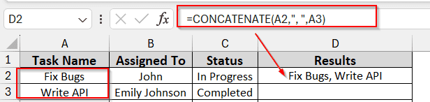
Combining cells in Excel may appeal to those who are more at ease using formulas. If necessary, you can merge the cells after first joining their values using the CONCATENATE function. Let’s say you have data in cells A2 and A3 of your Excel sheet, which you want to merge. Concatenate the two cells using the formula below to preserve the value in the second cell during the merging process:

Steps:

➤ Use the CONCATENATE() function in a new cell (D2).
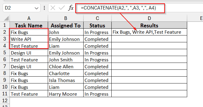
➤ To merge contents, use the above formula. Assuming we want to merge the first three cells,  the formula will be

➤ Drag the cells to generate the same formula for all cells in the D column.
➤ Click Merge and Center under the Alignment option to merge for proper alignment.

Cell values can be concatenated simply with the ampersand operator (&). This method is also another form of concatenating cells. However, it is simpler and easier to execute due to its short formula structure. If you want to join the texts of two cells, such as A1 and A2, you can use the formula below-

Steps:

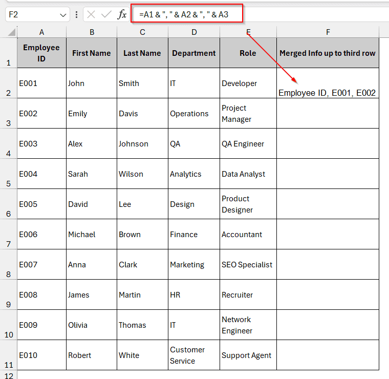
➤ Put the following formula in a blank cell:
=A1 & “, ” & A2 & “, ” & A3, where  cells in the range of A1 to A3 have to merged.
➤ To view the combined result, press Enter.

➤ Drag the cells to apply this formula to all the columns.
➤ Finally, combine the original cells by selecting Merge & Center under the Alignment option for proper alignment.

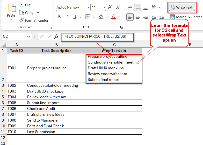
The TEXTJOIN function is also similar to the CONCATENATE function. The difference is that they have different parameters inside the formula. The main benefit of this function is that it strategically ignores empty spaces and ensures no data is lost using a specialized parameter. Assuming we want to merge cells B2 to B6, we can use the formula –

Here, the CHAR(10) indicates the line break, and the TRUE eliminates the empty cells.

Steps:

➤ Put the formula in the new cell (C2) using the cell range you want to join.
➤ Use the formula –
TEXTJOIN(CHAR(10), TRUE, B2:B6), where B2 to B6 are the cell range you want to join.
➤ After closing the parentheses, hit Enter.
➤ Wrap the text using the option of Wrap Text to merge the cells in under Alignment.

A VBA macro can automate cell merging without erasing data for huge datasets or repetitive activities. It mainly combines and merges large amounts of data, like comments, updates, notes, etc. Rather than using other methods that visually merge cells, this method intricately merges the content of the cell internally.

Steps:

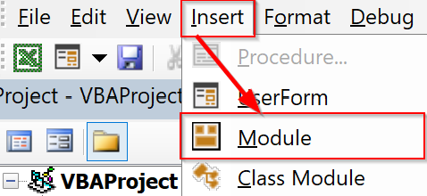
➤ To open the VBA editor, press the Developer Tab-> Visual Basic.
➤ From the Insert Tab, Select Module.

➤ Paste the following code into a newly added module:

Sub MergeCellWithoutLosingData()
    Dim cell As Range
    Dim combinedText As String
     For Each cell in Selection
        If cell.Value <> "" Then
            combinedText = combinedText & cell.Value & “ ”
Next cell
 With Selection
        .Merge
        .Value = Trim(combinedText)
        .WrapText = True
        .HorizontalAlignment = xlCenter
       .VerticalAlignment = xlCenter
    End With
End Sub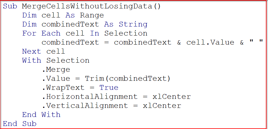

➤ Save and shut down the VBA editor.
➤ Choose which cell range to combine and select it
➤ Select Macros -> MergeCellsWithoutLosingData, and click Run.

➤ After that, the selected columns will look like the following:

Frequently Asked Questions (FAQS)

Is it possible to vertically merge cells in Excel without erasing all of the data?

Yes, but not when using Excel’s built-in Merge & Center feature. Excel automatically deletes all other data and only saves the contents of the top cell. You should merge the cells after combining the contents of each cell using formulas like TEXTJOIN, CONCAT, or other functions to preserve all data.

What is the Excel shortcut for merging and centering cells?

First, click on the Alt key to display all the ribbon commands. Press H and M from there to merge and center the cell’s contents.

When I merge cells in Excel, why does it erase data?

This is because Excel’s built-in merging features, such as Merge & Center, are made to preserve just the data in the top-left cell inside the chosen range. Unless you first combine them using a formula, the values in other cells are erased.

Will sorting or filtering in Excel be impacted by cell merging?

Sorting and filtering in Excel can be impacted while merging cells. Because they span several rows or columns, merged cells may pose issues with sorting and filtering. Avoid merging data that has to be sorted or filtered. Instead, use concatenation formulas to display the combined material in an assistance column.

Which versions of Excel are compatible with the TEXTJOIN function?

Excel 2016 and later versions, including Microsoft 365, support the TEXTJOIN function. You need to use alternatives like CONCATENATE, the ampersand operator, or a VBA script if you are using Excel 2013 or older.

Wrapping Up

In this article, we looked at several useful techniques for safely combining cells vertically, such as using the simplest ways like the Justify option and even complex VBA coding methods.. These methods will assist you in maintaining data integrity while creating a more streamlined layout, whether you’re organizing complex data, integrating notes, or consolidating lists.