When building smart Excel forms or dashboards, dropdown lists that change based on another cell can dramatically improve usability. Whether you’re managing categories, subcategories, or dynamic data, Excel’s data validation tools offer effective ways to automate and restrict input.
In this article, you’ll learn how to apply Data Validation in Excel based on another cell using practical techniques. From simple formulas to dynamic dropdowns, these methods enhance accuracy and user control.
Steps to apply data validation based on another cell in Excel:
➤ Select range A2:A4 and name it Fruit using Formulas tab >> Define Name >> Click OK.
➤ Do the same for Vegetable (B2:B4) and Grain (C2:C4).
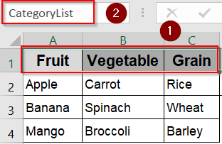
➤ Then Select header row A1:C1 and name it CategoryList using the Name box next to Formula Bar.
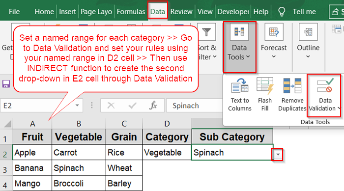
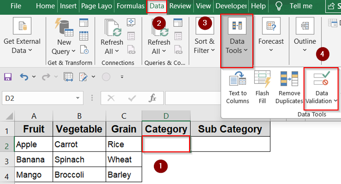
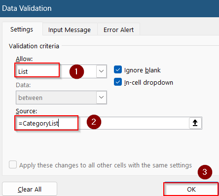
➤ Select any blank cell like D2 and go to the Data tab >> Data Validation under Data tools. Set Allow to List and inside Source box, type: =CategoryList
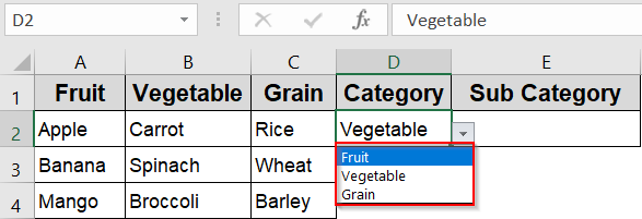
➤ Click OK. This will create your first drop-down level in D2 cell.
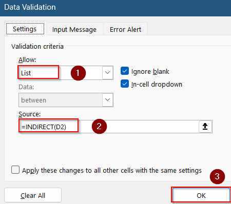
➤ Select cell E2 (Sub Category) >> Go to the Data tab >> Data Validation under Data tools. Choose List under “Allow” and in the Source field, enter: =INDIRECT(D2) and click OK.
Create a Simple Dependent Drop‑Down List
This method is great when you have fixed categories like Fruit, Vegetable, or Grain. Using named ranges and the INDIRECT function, you can build dynamic dropdowns that change based on another cell.
Steps:
➤ Select range A2:A4 and go to Formulas tab >> Define Name.
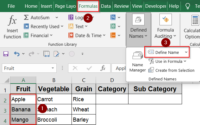
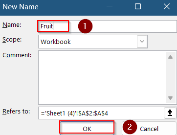
➤ Name it Fruit and click OK.
➤ Do the same for Vegetable (B2:B4) and Grain (C2:C4).
➤ Then Select header row A1:C1 and name it CategoryList using the Name box next to Formula Bar.
➤ Select any blank cell like D2 and go to the Data tab >> Data Validation under Data tools.
➤ Set Allow to List and inside Source box, type:
=CategoryList
➤ Click OK. This will create your first drop-down level in D2 cell.
➤ Select cell E2 (Sub Category).
➤ Go to the Data tab >> Data Validation under Data tools.
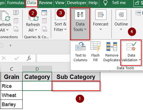
➤ Choose List under “Allow”.
➤ In the Source field, enter:
=INDIRECT(D2)
To support categories with spaces such as “Red Fruit”, you can use this:
=INDIRECT(SUBSTITUTE(D2,” “,”_”))
➤ Click OK. This will create your second drop-down level in E2 cell.
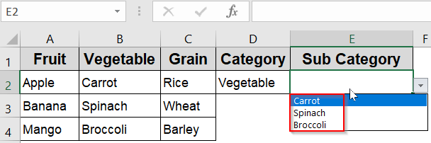
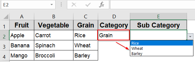
Now, when D2 is selected as “Vegetable“, E2 shows values from the named range Vegetable. If you select Fruit in Category, the drop-down for column E will change automatically.
Build Multi‑Level Dependent Drop‑Downs
This method builds on the previous one, allowing you to create a three-level hierarchy (e.g., Category >> Subcategory >> Items). You’ll use named ranges by combining first and second dropdown values which is perfect for complex, layered inputs.
Steps:
➤ Follow previous method to build Category and Subcategory dropdowns.
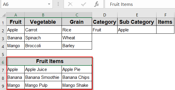
➤ Then, add a helper for each category item. For example, we have created a helper for Fruit Items ranging from A7:C9.
➤ Select B7:C7 cell and name it FruitApple inside the Name box next to the formula bar.
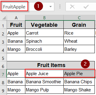
➤ Repeat the same steps for others such as name it FruitBanana for B8:C8 and name it FruitMango or B9:C9.
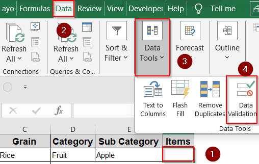
➤ Select F2 cell and go to the Data tab >> Data Validation under Data tools.
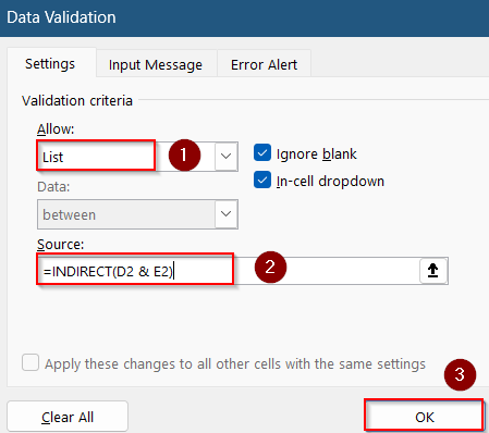
➤ Set Allow to List and type in Source:
=INDIRECT(D2 & E2)
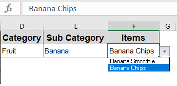
This creates a three-level cascading dropdown, where each selection influences the next.
IF Function for Conditional Lists (No Named Ranges)
If you’re only working with a few fixed categories, this method avoids named ranges altogether. It uses IF function statements to manually route each category to its matching list.
Steps:
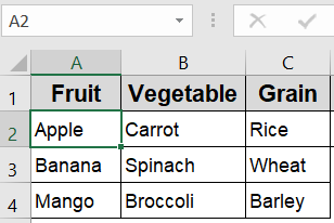
➤ List each category’s values such as Fruit, Vegetable and Grain vertically in columns A, B, and C respectively.
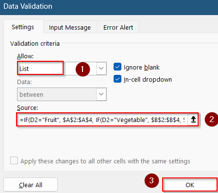
➤ Select any blank cell like E2 where you want the dependent dropdown and go to the Data tab >> Data Validation under Data tools.

➤ Set “Allow” to List.
➤ In the Source box, enter:
=IF(D2=”Fruit”, $A$2:$A$4, IF(D2=”Vegetable”, $B$2:$B$4, $C$2:$C$4))
➤ Click OK.
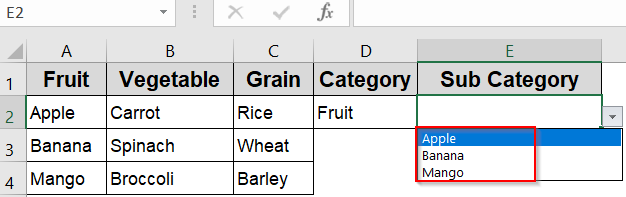
Now, if you type “Fruit” in D2 cell, E2 will show Apple, Banana, Mango. If “Vegetable” is entered in D2, it’ll show Carrot, Spinach, Broccoli in E2, which makes the drop-down dynamic based on entry in another cell.
Try Custom Data Validation Formula (Advanced Logic)
Instead of dropdowns, this approach prevents wrong manual input using a custom formula. It blocks anything not found in the sublist matching the selected category.
Steps:
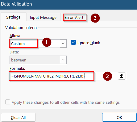
➤ Select cell E2 where the sub-category goes.
➤ Go to the Data tab >> Data Validation under Data tools.

➤ Under “Allow,” choose Custom.
➤ In the Formula field, enter:
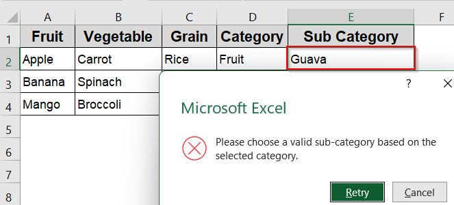
=ISNUMBER(MATCH(E2,INDIRECT(D2),0))
➤ Go to the Error Alert tab and add a message like:
“Please choose a valid sub-category based on the selected category.”
➤ Click OK.
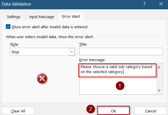
Now, users cannot enter invalid values in E2 that don’t match the selected category in D2 such as the entry Guava which does not exist in column A.
Using VBA for Dynamic Data Validation
This VBA method auto-refreshes the dropdown cell every time reference cell changes which makes it great for forms or dashboards where dropdowns should react instantly without manual data validation reset.
Steps:
➤ Press Alt + F11 to open the VBA Editor.
➤ In the Project pane, double-click the sheet you’re working on (e.g., Sheet1).
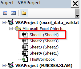
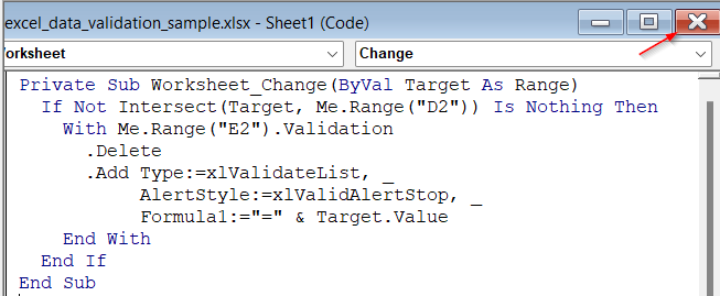
➤ Paste the following code into the sheet module:
Private Sub Worksheet_Change(ByVal Target As Range)
  If Not Intersect(Target, Me.Range("D2")) Is Nothing Then
    With Me.Range("E2").Validation
      .Delete
      .Add Type:=xlValidateList, _
           AlertStyle:=xlValidAlertStop, _
           Formula1:="=" & Target.Value
    End With
  End If
End Sub
➤ Close the editor and return to Excel.
Now, when you change D2, Excel automatically adjusts E2’s dropdown to the matching list such as entering Grain in column D.
Frequently Asked Questions
Can I use dependent dropdowns between different sheets in Excel?
Yes, but you must use named ranges for data on other sheets since direct references won’t work in data validation’s Source box unless inside a named formula.
What if my category names contain spaces?
Use the SUBSTITUTE function inside INDIRECT, like INDIRECT(SUBSTITUTE(D2,” “,”_”)), so Excel reads “Red Fruit” as “Red_Fruit” to match your named ranges properly.
Will Excel Tables automatically expand dropdown options when I add more data?
Yes, if you use structured references with INDEX/MATCH inside named ranges. Tables automatically grow, and dependent dropdowns will reflect those new entries without manual updates.
Do I have to use VBA for dynamic dropdowns?
No, VBA is optional. It’s helpful for real-time dropdown updates but isn’t necessary if you’re using INDIRECT, IF, or table formulas for dynamic lists.
Wrapping Up
In this tutorial, we learned how to create Excel data validation based on another cell using methods like functions like INDIRECT, IF, MATCH, and even VBA. Whether you’re building a multi-level dropdown or preventing invalid inputs, each approach can help make your spreadsheets more dynamic and error-proof. Feel free to download the practice file and share your feedback.