Managing a growing list of data like employee records, customer orders, or product catalogs can quickly become overwhelming. Manually scrolling through hundreds or even thousands of rows isn’t just time-consuming, it’s inefficient. That’s why creating a searchable database in Excel is a smart move.
In this article, you’ll learn how to build a searchable Excel database using easy-to-follow methods from simple filters to dynamic search boxes and formula-driven search tools. Whether you’re working with a small table or a large dataset, these steps will help you find what you need quickly and accurately.
Steps to create a searchable database in Excel:
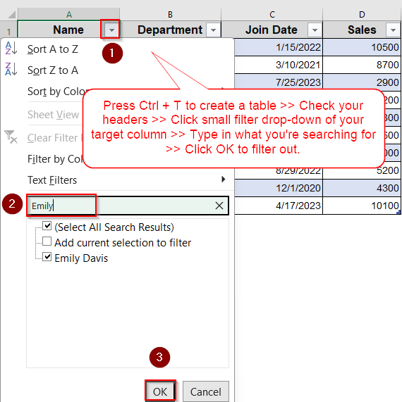
➤Press Ctrl + T to create a table.
➤Make sure “My table has headers” is checked.
➤Click the small filter drop-down at the side of your target column and type your keyword.
➤Click OK to filter out.
Use Filter to Search in Excel Table
If you’re just starting out and want a quick way to make your Excel data searchable, the built-in filter option is your best option. It’s ideal for simple datasets and requires no formulas or special tools. Once your data is in a table format, Excel provides instant dropdown filters that let you search and display relevant rows with ease.
Steps:
➤ Select your data range and press Ctrl + T or go to Insert tab >> Table to convert it into a table. Make sure “My table has headers” is checked.
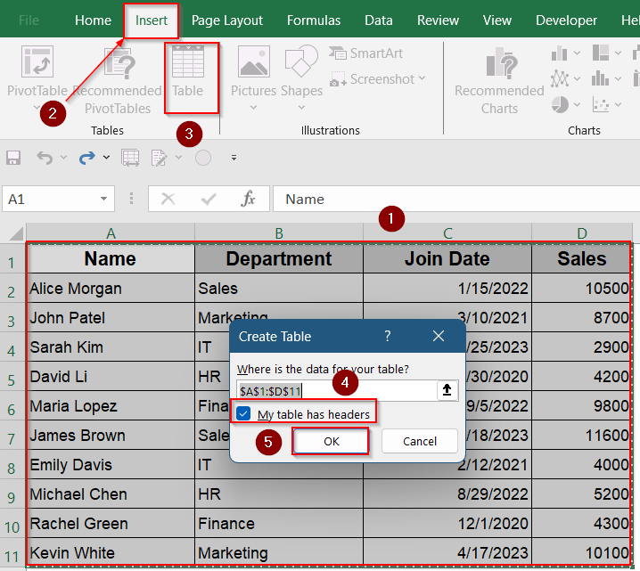
➤ You’ll see filter dropdown arrows appear on each column header.
➤ Click the dropdown arrow on the column you want to search in and go to the search box to filter your data.
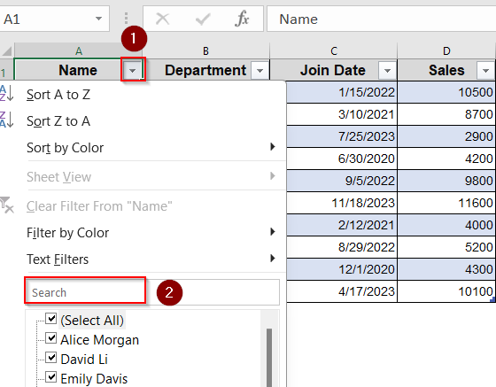
➤ In the search box that appears, type the keyword or value you’re looking for such as Emily.
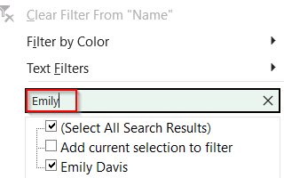
➤ Excel will instantly show only the rows that match your query.
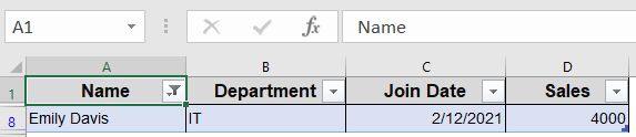
This method works well for simple searches within individual columns.
Create a Dynamic Search Box with Formulas
If you want your database to be interactive by showing filtered results instantly as the user types, then this method is for you. Using array formulas, you can build a dynamic search tool that updates in real-time. This is especially helpful when you’re dealing with mid-sized datasets and want to avoid manual filtering.
Steps:
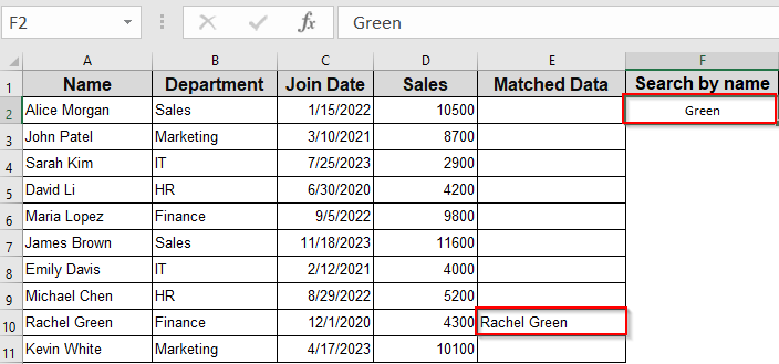
➤ In a blank cell (say F1), type a label: Search by Name.
➤ In cell F2 allow user input which means that cell will be your search box.
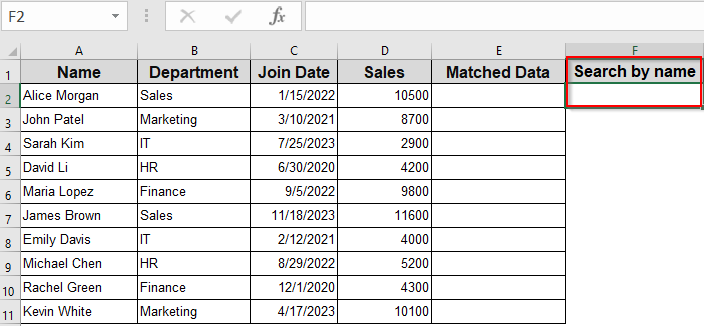
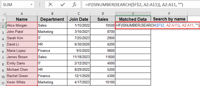
➤ In the Matched Data column, enter the following array formula in E2 cell to extract matching records:
=IF(ISNUMBER(SEARCH($F$2, A2:A11)), A2:A11, “”)
➤ Press Ctrl + Shift + Enter to activate the array formula (if using older Excel versions). New Excel versions handle it with just Enter.
➤ Drag the formula across and down to fill the search results.
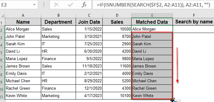
Now, any partial name typed in F2 will return all matching rows from your dataset.
Combine Search with Drop-Down List and VLOOKUP
Want a cleaner, more controlled way to search? Try using a drop-down list combined with VLOOKUP to instantly retrieve detailed information. This is especially useful for dashboards, employee lookup tools, or inventory sheets where the search term is predefined like an ID or name.
Steps:
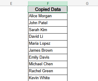
➤ Copy the names from column A (A2:A11) to column F (F2:F11) to prepare a unique name list.
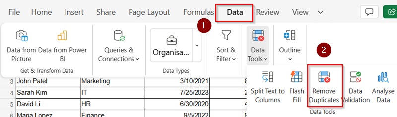
➤ Go to the Data tab >> Click Remove Duplicates if needed.
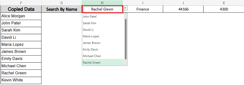
➤ To create the Drop-Down Menu, click on an empty cell such as H1 >> Go to Data >> Data Validation.
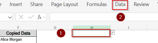
➤ In the dialog box, choose List under “Allow.”
➤ For the Source, select the range F2:F11 using the small button at the right and click OK.

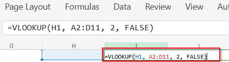
➤In cell I1, enter this formula to fetch Department using VLOOKUP:
=VLOOKUP(H1, A2:D11, 2, FALSE)
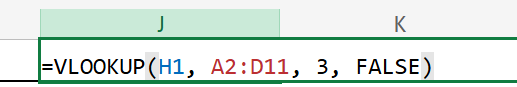
➤ In cell J1, enter this formula to fetch Join Date using VLOOKUP:
=VLOOKUP(H1, A2:D11, 3, FALSE)
➤ In cell K1, enter this formula to fetch Sales using VLOOKUP:
=VLOOKUP(H1, A2:D11, 4, FALSE)

Now, when you select a name from the drop-down in H1, the corresponding department, join date, and sales info will automatically populate in cells I1, J1, and K1.
Use Conditional Formatting for Visual Filtering
If you don’t want to hide non-matching rows but still want to highlight search results, conditional formatting is a great choice. It allows you to visually scan and identify matches without altering the structure of your dataset.
Steps:
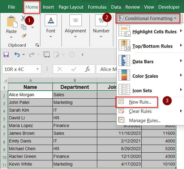
➤ Select your entire dataset (e.g., A2:D11).
➤ Go to Home >> Conditional Formatting >> New Rule.
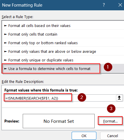
➤ Choose Use a formula to determine which cells to format.
➤ Enter the formula (assuming search cell is F1 and you’re matching names in column A):
=ISNUMBER(SEARCH($F$1, A2))
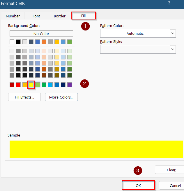
➤ Click Format, set a fill color (e.g., light yellow), and click OK.
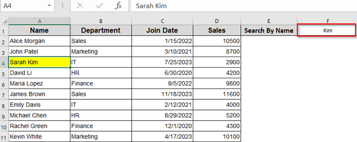
Now, any row with a match will be visually highlighted.
Frequently Asked Questions
Can I search multiple columns at once?
Yes, you can create a helper column that combines multiple fields (like Name and Department). Then, use that column for lookup or filtering to enable multi-column searches.
Will the formulas still work if my data updates regularly?
Yes, as long as you expand the ranges or use Excel Tables (which auto-expand). You can also make your formulas dynamic using INDEX, MATCH, or FILTER.
Is there a way to create a search box without formulas or coding?
Yes. You can use Excel’s built-in Filter feature. Click the drop-down in any column header and type in the search box to find matching values instantly.
Does Excel support real-time search like a web app?
Not directly. However, with clever use of formulas or VBA code tied to Worksheet_Change events, you can mimic a real-time search experience in Excel quite effectively.
Wrapping Up
In this tutorial, we learned how to create a searchable Excel database using both a dynamic formula-based search box and a cleaner drop-down list paired with VLOOKUP. You saw how each method helps retrieve specific records instantly, whether you’re typing partial names or selecting from a list. Feel free to download the practice file and share your feedback.