If you’re tracking project timelines, employee onboarding, or event planning in excel you can calculate the number of weeks between two dates. If we know the exact number of weeks it can help us with resource allocation, scheduling, time tracking. And many more further applications.
To calculate number of weeks between two dates Excel, follow these steps:
➤ Enter your start and end dates in two separate cells.
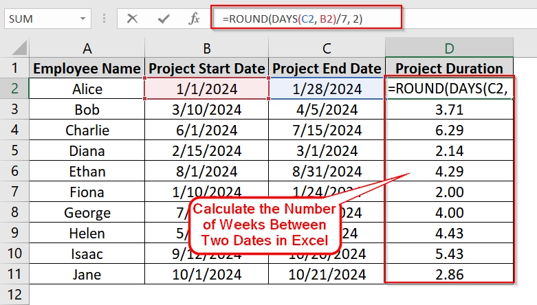
➤ Use the formula =ROUND(DAYS(C2, B2)/7, 2)
➤ Press Enter to view the number of completed weeks between the two dates.
In this article, we’ll explain multiple Excel methods that can calculate weeks between dates. We will use formulas like INT, DATEDIF, and TODAY(), with real life data examples.
Quick Video Tutorial: Number of Weeks Between Two Dates in Excel
Using the DAYS Function and Division to Calculate Weeks Between Two Dates
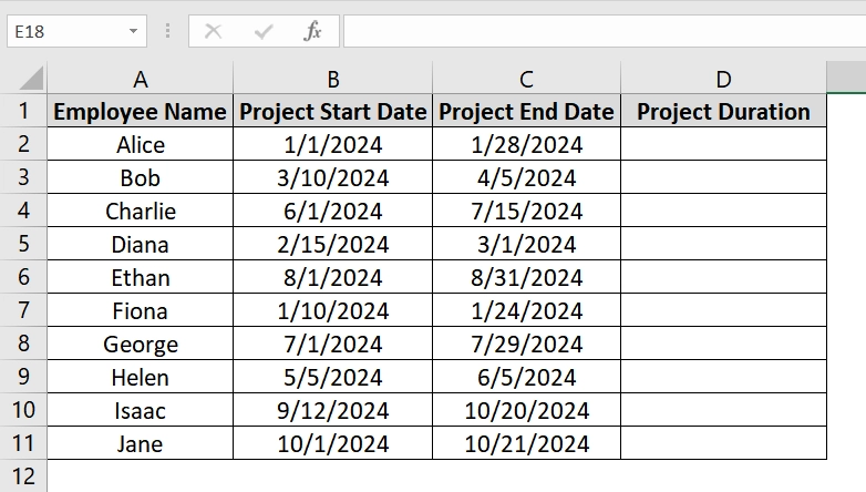
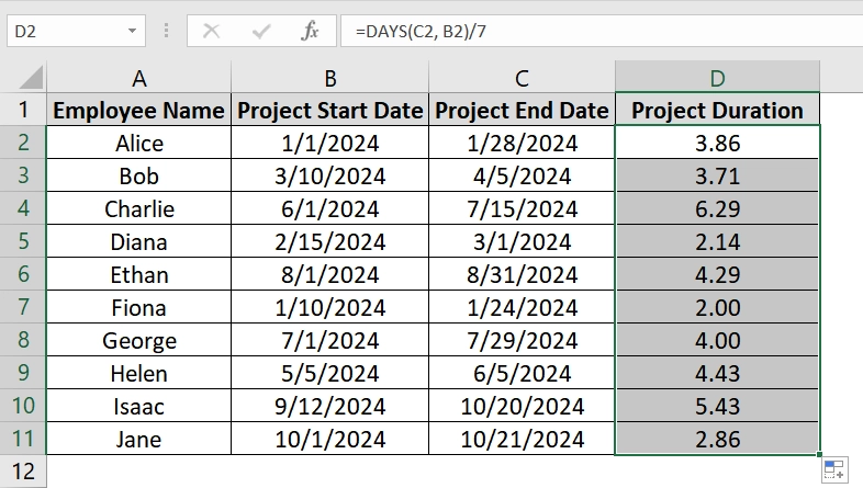
This method uses Excel’s DAYS function to calculate the number of days between two dates and then divides the result by 7 to get the number of weeks. It is best used when you need a decimal value that shows the total weeks, including partial weeks (e.g., 3.5 weeks). Here we have taken a situation where some employees are assigned to a project. We have a dataset containing Employee Name, Project Start Date, Project End Date. We need to calculate the project duration in Weeks.
Steps:
➤ Open up your excel datasheet. You can also use our demo excel worksheet for practice. Just download and open the excel file and navigate to sheet 1.
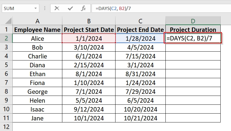
➤ In cell D2, enter the following formula to calculate the number of weeks between the dates in C2 (end date) and B2 (start date):
=ROUND(DAYS(C2, B2)/7, 2)
This formula will return a decimal value indicating the total number of weeks between the two dates, including any part of a week.
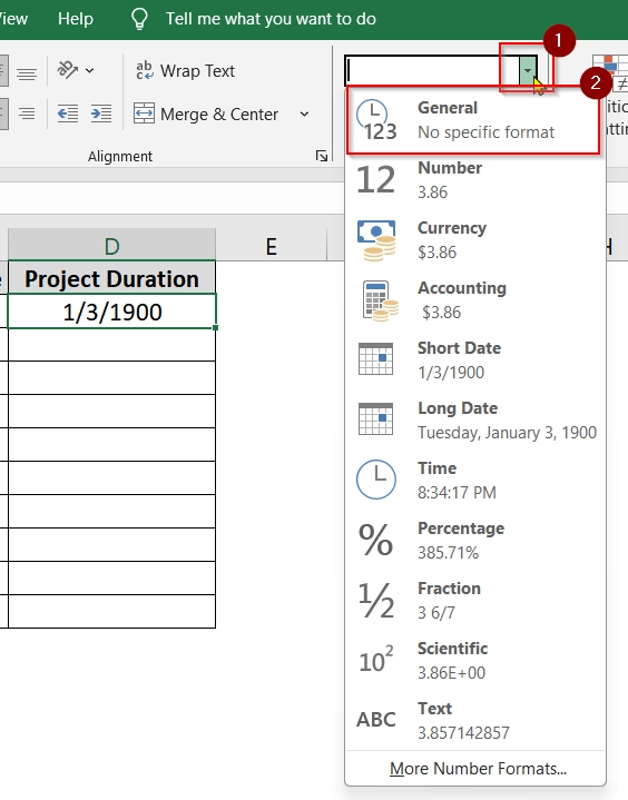
➤ Format the cell as General. To formate go to Home and then select the General under the Number group.
➤ Drag the formula down from cell D2 to the rest of the rows in Column D to apply the same calculation for each employee.
Note:
➧ This method counts only the number of calendar weeks, not workweeks.
➧ The result includes partial weeks (e.g., 3.5 = 3 weeks and 3.5 days).
Applying INT and DAYS Function To Calculate Full Weeks Between Two Dates
This method will calculate the total number of complete weeks between two dates in Excel. We use it for only full weeks (7-day periods) are needed. That can be for tracking weekly training modules, employee shifts, or maybe project billing periods.
Steps:
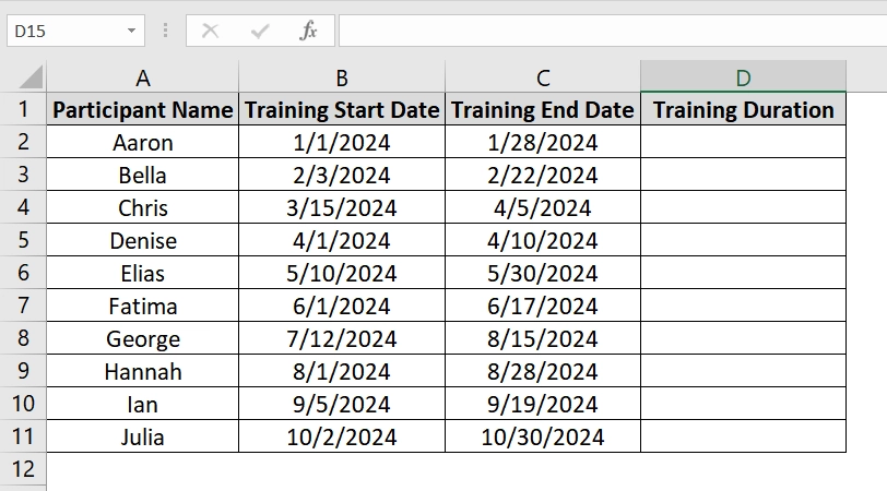
➤ Open up your excel datasheet. Here we have dataset that includes:
- Column A: Participant Name
- Column B: Training Start Date
- Column C: Training End Date
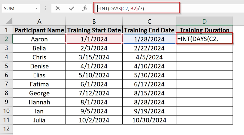
➤ In cell D2, input the following formula and click Enter.
=INT(DAYS(C2, B2)/7)
➤ Use the fill handle to drag the formula down from cell D2 to apply it to the rest of the rows in Column D.

➤ (Optional): If you want to prevent errors when dates are missing or wrongly ordered, use an improved formula:
=IF(AND(ISNUMBER(B2), ISNUMBER(C2), C2>B2), INT(DAYS(C2, B2)/7), “”)
This formula checks:
- Both start and end dates are valid numbers.
- End date is after the start date.
- If the check fails, it leaves the cell blank.
Note:
➧ This method excludes any partial weeks. For example, 13 days = 1 full week, not 1.86.
➧ To include partial weeks, use the method =DAYS()/7
Let The Simple Subtraction and Division To Calculate Weeks Between Two Dates
Simple Subtraction and Division method is an easy and quick way to calculate the number of weeks (including partial weeks) between two dates in Excel. It’s used when you want a precise decimal-based result instead of rounding to whole weeks for example in cases like payroll calculations, resource planning etc.
Steps:
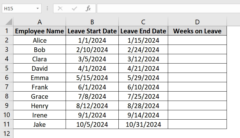
➤ Open an Excel workbook. We have a worksheet where-
- Column A: Employee Name
- Column B: Leave Start Date
- Column C: Leave End Date
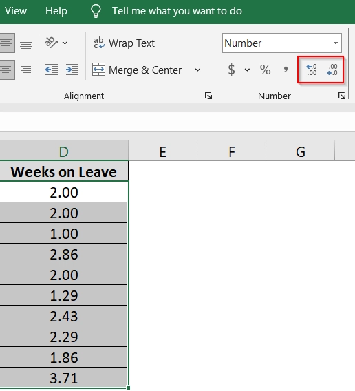
➤ In cell D1, type the header: Weeks on Leave . This will be our result column.
➤ Click cell D2 and enter the following formula:
=(C2 – B2)/7
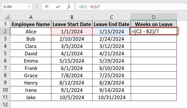
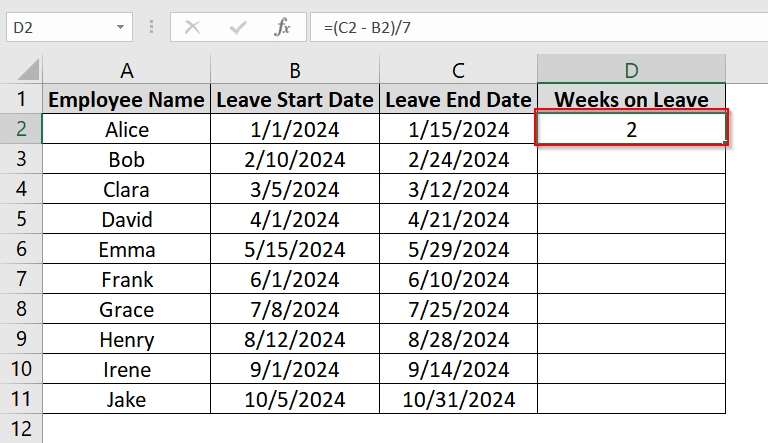
➤ Press Enter. You will now see the number of weeks (with decimals) for the first row.
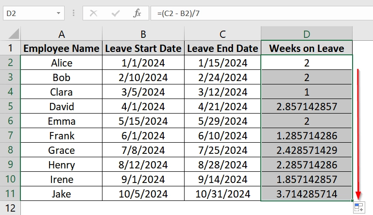
➤ Drag the fill handle (small square at the bottom-right of cell D2) down through the rest of the column to apply the formula to all rows.
➤ (Optional): Format the result column (Column D) to show only two decimal places. Select the column. Go to Home > Number. Here you will see these two icons to increase or decrease decimal places. Adjust as you need by clicking on it.
Note:
➧ This method includes partial weeks. For instance, a leave of 10 days will show as approximately 1.43 weeks.
➧ Use this method when fractional weeks matter, such as for salary deductions, resource booking, or average work periods.
➧ If you only want whole weeks, use =INT((C2 – B2)/7)
Implementing DATEDIF Function To Calculate Weeks Between Two Dates
This method uses the DATEDIF function to count the number of days between two dates and then divides the result by 7 to get the number of weeks. It’s suitable if you prefer a function based solution and want a decimal result.
Steps:
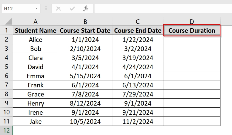
➤ Open the Excel spreadsheet.
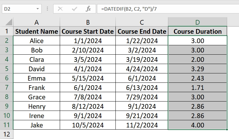
➤ In cell D1, type the header: Course Duration. This will be our result column.
➤ Click on cell D2 and enter this formula:
=DATEDIF(B2, C2, “D”)/7
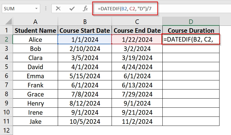
➤ Press Enter. The result will show the number of weeks in decimal format (e.g., 3.14). If you see a date, format the cell as General from Home> Number
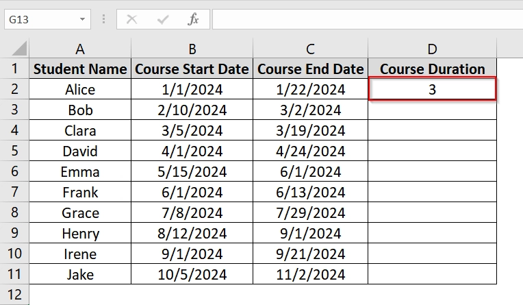
➤ Use the fill handle to drag the formula down through the rest of the rows (e.g., D2 to D11). Excel will automatically adjust the cell references for each row.
Note:
DATEDIF is a hidden but supported function in Excel; it won’t appear in formula suggestions but works reliably.
Use the TODAY Function To Calculate Weeks from Start Date to Today
TODAY function can calculate the number of full weeks that have passed from a specific start date until the current date. It’s useful in scenarios such as employee tenure tracking where the end date keeps changing (i.e., always today). You should use this method for real-time tracking in dashboards or weekly status reports.
Steps:
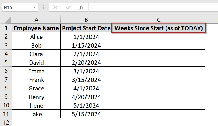
➤ Open your Excel sheet. We have used Column A for Employee Name, Column B for Project Start Date.
➤ In Column C, add the header Weeks Since Start (as of TODAY) in cell C1.
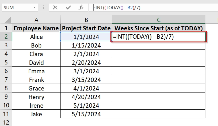
➤ Click on cell C2 and enter the formula:
=INT((TODAY() – B2)/7)
Here,
- TODAY fetches the current date dynamically.
- B2 is the start date.
- The subtraction returns the total number of days between today and the start date.
- Dividing by 7 converts days into weeks.
- INT() removes any partial week, giving a whole number of completed weeks.
➤ Press Enter to calculate the weeks passed for the first entry.
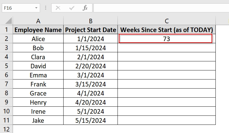
➤ Use the fill handle to drag the formula down to the remaining rows (C3 to C11).

Note:
➧ This method auto-updates every day when you open the sheet, as TODAY() always returns the current system date.
➧ Use INT if you’re only interested in full weeks. If you want decimal precision (e.g., 4.29 weeks), use (TODAY() – B2)/7 without INT().
Frequently Asked Questions (FAQs)
How do I calculate the number of weeks between two dates in Excel?
Use the formula =INT((End_Date – Start_Date)/7) to get complete weeks.
How to calculate week number in Excel?
Use =WEEKNUM(Date) to get the week number of a particular date.
What is the formula for DATEDIF?
=DATEDIF(Start_Date, End_Date, “D”) gives the number of days. Divide by 7 to get weeks.
What is the formula for 2 weeks from date in Excel?
Use =Start_Date + 14 to get the date 2 weeks from a given date.
Concluding Words
The most effective way to calculate the number of weeks between two dates in Excel is by using the INT((End_Date – Start_Date)/7) method or its dynamic variant with TODAY(). This method is good for both fixed and ongoing timelines. It can ensure accurate weekly reporting. Beside this, we have shown many other methods. You can choose whichever fits your needs. Also, if you have any questions please let me know.