Creating a drop-down list in Excel is one of the most effective ways to guide user input, minimize data entry mistakes, and standardize your spreadsheets. Whether you’re managing product categories, task statuses, or employee roles, a well-crafted drop-down list can make your workbook more interactive and efficient.
In this article, you’ll learn several ways to create drop-down lists directly from tables ranging from static to dynamic lists. Each method includes step-by-step instructions, so you can confidently apply the one that fits your Excel project best.
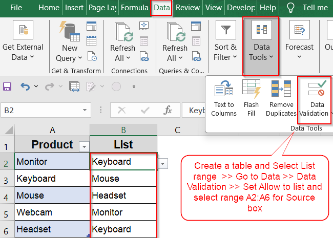
Steps to create a drop-down list from a Table in Excel:
➤ Create a table pressing Ctrl + T .
➤ Select the cells such as B2:B6 where the drop-down should appear.
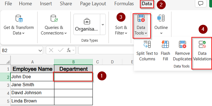
➤ Go to Data >> Data Validation under Data Tools on the ribbon.
➤ In the Settings tab set Allow to List and select the range A2:A6 or table column using the small button at the left in the Source box.
➤ Click OK.
Convert List to an Excel Table for Auto-Expanding Source
This is the fastest way to build a drop-down list from a column of values. When you convert a range into an Excel Table, the drop-down list updates automatically as you add more items which is ideal for structured, frequently updated datasets.
Steps:
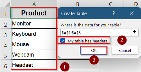
➤ Create or ensure your list values are in a contiguous range such as A2:A6 or in a column of a table. To turn your data into a Table, use Ctrl + T and check your headers. Then, click OK.
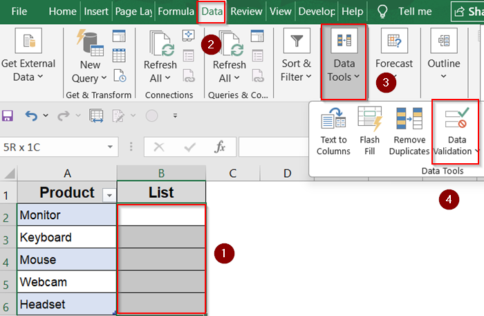
➤ Select the cells such as B2:B6 where the drop-down should appear.
➤ Go to Data >> Data Validation under Data Tools on the ribbon.
➤ In the Settings tab set Allow to List and select the range A2:A6 or table column using the small button at the left in the Source box.
➤ Click OK.
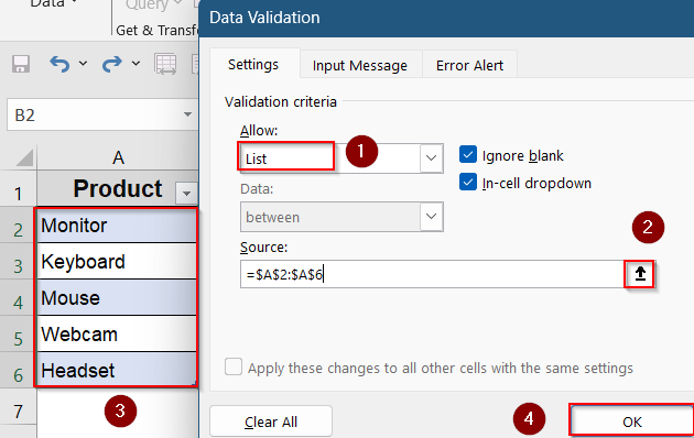
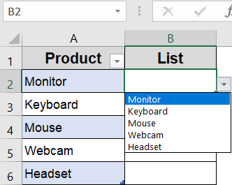
➤ You will find a drop-down arrow next to the selected cells using your Table data as the source.

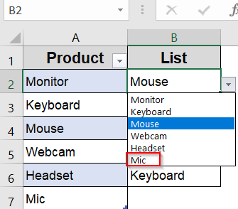
Now, when you add new rows to the table, the drop-down includes them automatically such as Mic in A7 cell.
Set Up Named Range for Portability Across Sheets
If you plan to use the same list across multiple sheets, naming your Table columns makes referencing clean and portable. This method avoids errors from direct range references and keeps your formulas readable.
Steps:
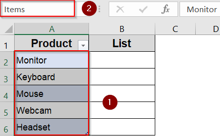
➤ Select your list values (A2:A8).
➤ In the Name Box (left of the formula bar), type a name like Items.
➤ Press Enter to create the named range.
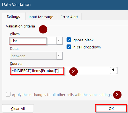
➤ Go to Data >> Data Validation under Data Tools on the ribbon.

➤ In the Settings tab set Allow to List and in the Source box type:
=INDIRECT(“Items[Product]”)
➤ Click OK.
The named range functions like a portable table column, usable anywhere in the workbook.
Apply a Dynamic Named Range with OFFSET Function
If you frequently add or remove items, a dynamic named range using OFFSET and COUNTA function auto-adjusts to include only populated cells.
Steps:
➤ Suppose your list starts at Sheet3!A2.
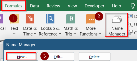
➤ Click Formulas tab >> Go to Name Manager on the ribbon >> Click New.
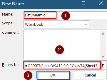
➤ Give it a Name it such as ListDynamic.
➤ In Refers to box, enter:
=OFFSET(Sheet3!$A$2,0,0,COUNTA(Sheet3!$A:$A)-1,1)
➤ Click OK.
➤ Close the Name Manager dialog box.
➤ Go to Data >> Data Validation under Data Tools on the ribbon.

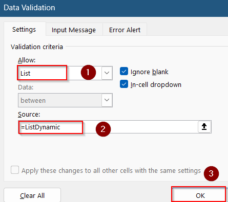
➤ In the Settings tab, set Allow to List and in the Source box type:
=ListDynamic
➤ Click OK.
Your drop-down list will now grow or shrink automatically when you update the source list.

Pull Drop-Down List from Table in Another Sheet
You can also build drop-down lists from tables stored on a separate worksheet. This is especially useful when your data source is stored or maintained independently.
Steps:
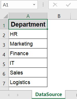
➤ Create a sheet called DataSource where you will list your drop-down data.
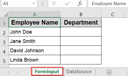
➤ Add a new sheet called FormInput where the drop-down should appear.
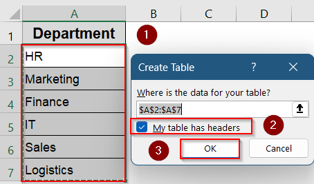
➤ Go to the DataSource sheet and select cells A1:A7, including the header.
➤ Press Ctrl + T to create a Table and make sure “My table has headers” is checked.
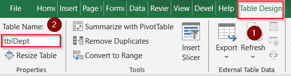
➤ Go to the Table Design tab and rename the table to tblDept.
➤ Now go to the FormInput sheet and select cell B2.
➤ Click on the Data tab and choose Data Validation under Data tools on the ribbon.
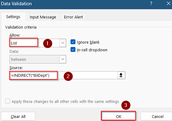
➤ In the dialog, set Allow to List.
➤ Inside Source box, type:
=INDIRECT(“tblDept”)
➤ Click OK.
➤ As the drop-down sign appears, you can now drag down using the AutoFill handle to add a drop-down list for the rest of the cells and select the correct value according to your data.
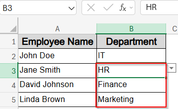
This method ensures that whenever you add a new department in the DataSource sheet such as Customer Support, the drop-down updates automatically.
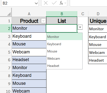
Use UNIQUE Function for a Dynamic List Without Duplicates (Excel 365/2021)
With newer versions of Excel, the UNIQUE function spills unique items from a table or range, which removes duplicates from your data. This method is perfect for building a dynamically updating drop-down without helper columns.
Steps:
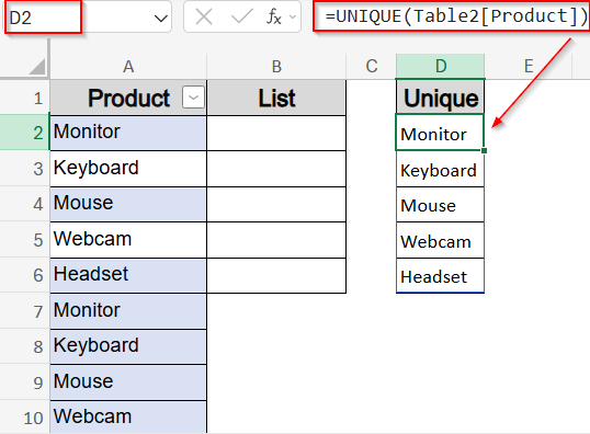
➤ Suppose your table column is A2:A14.
➤ In an empty cell (e.g. D2), enter:
=UNIQUE(Table2[Product])
➤ The list spills down populated values.
➤ Select range B2:B6 >> Go to Data >> Data Validation under Data Tools on the ribbon.

➤ In the Settings tab, set Allow to List and in the Source box type
=$D$2#
➤ Click Apply to save changes.
This drop-down always shows unique entries and updates as the source table changes.
Frequently Asked Questions
Can I source a drop-down list from another worksheet?
Yes, you can use a named range or table referenced workbook-wide. Alternatively, you can include the sheet name directly in the following format: =Sheet2!$A$2:$A$10
Can I use a list from another workbook?
Yes. First, define named dynamic ranges in each workbook and then reference the source list’s name in the destination workbook’s Data Validation.
How do I allow users to enter custom values?
In Data Validation, go to Error Alert, uncheck “Show error alert after invalid data is entered”. This converts your drop-down into an editable combo box while preserving suggestions.
Wrapping Up
In this tutorial, we learned multiple ways to create a drop-down list from a table in Excel starting from simple static tables to dynamic named ranges, table references across sheets, and the modern UNIQUE function. Each method offers flexibility depending on how static or dynamic your source data is. Feel free to download the practice file and share your feedback.