A dynamic dependent drop-down list in Excel lets you control the items shown in one drop-down based on the selection in another. This functionality is perfect for creating smarter, interactive spreadsheets. It works well for data entry forms, inventory tools, or dashboards. For example, selecting a category like “Fruits” in one cell can automatically filter the second drop-down to show only related items like “Apple,” “Mango,” or “Banana.”
In this article, you’ll learn how to create dynamic dependent drop-down lists in Excel using structured tables, formulas, and named ranges. Each method is designed to make your spreadsheets more flexible, accurate, and user-friendly. You will see how to set up multiple dropdowns, expanding lists, and alphabetically sorted selections.
Steps to create a dependent drop-down list in Excel:
➤ Create named ranges for each category. For example, select B2:B4 and name it Fruits (matching the label in A2). Repeat for each category.
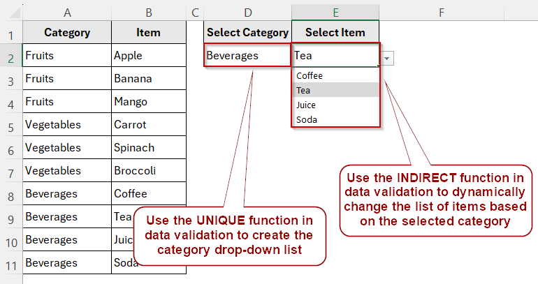
➤ In D2, set up the first drop-down by using this formula: =UNIQUE(A2:A11), this lists all category names.
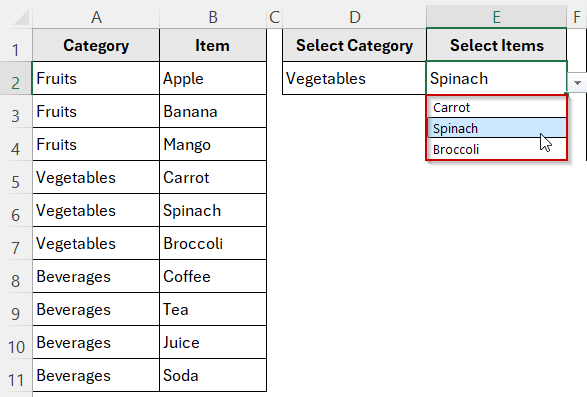
➤ In E2, set up the second drop-down using =INDIRECT(D2), which references the named range that matches the selected category.
➤ Now, when you select “Fruits” in D2, E2 will show Apple, Banana, and Orange.
Create a Dependent Drop-Down That Updates Automatically
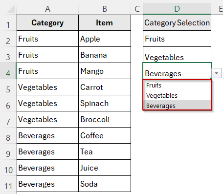
A dependent drop-down list allows the options in one cell to change dynamically based on the selection made in another cell. This is useful when you want users to first choose a category, such as “Fruits,” and then see only the relevant items like “Apple,” “Banana,” or “Mango” in the next dropdown. This method ensures that your form or worksheet stays accurate and easy to use.
Steps:
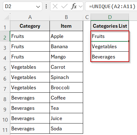
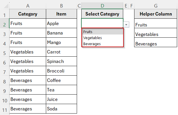
➤ Create a unique list of categories. In D2, enter the formula:
=UNIQUE(A2:A11)
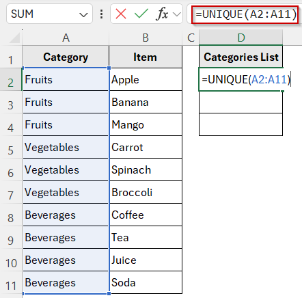
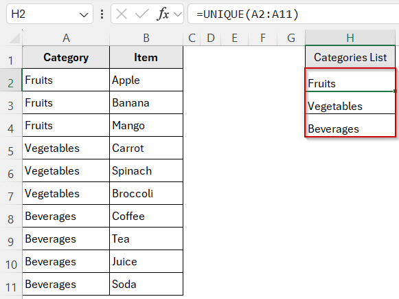
This will extract all main categories such as Fruits, Vegetables, and Beverages.
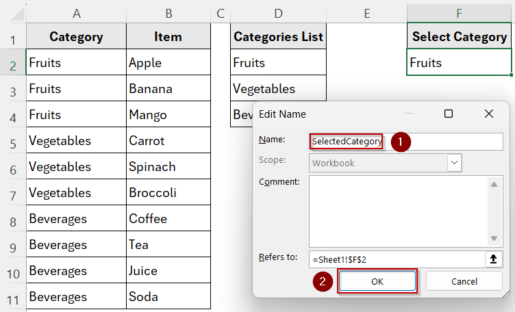
➤ Name the input cell where users will select a category. For example, in F2, enter: =D2
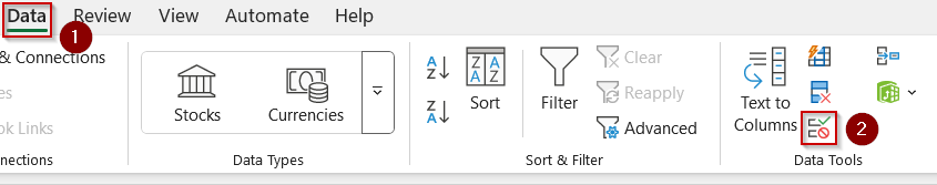
➤ Then go to Formulas >> Name Manager.
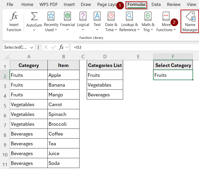
➤ Name this cell SelectedCategory.
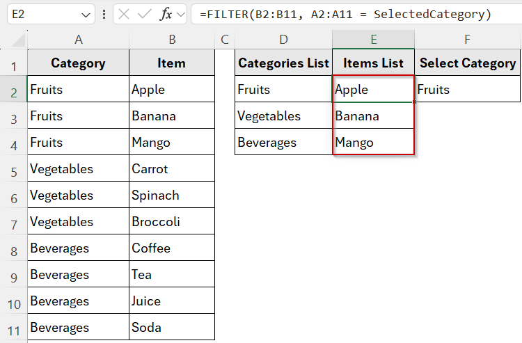
➤ Build the filtered list of items. In E2, enter the formula:
=FILTER(B2:B11, A2:A11 = SelectedCategory)
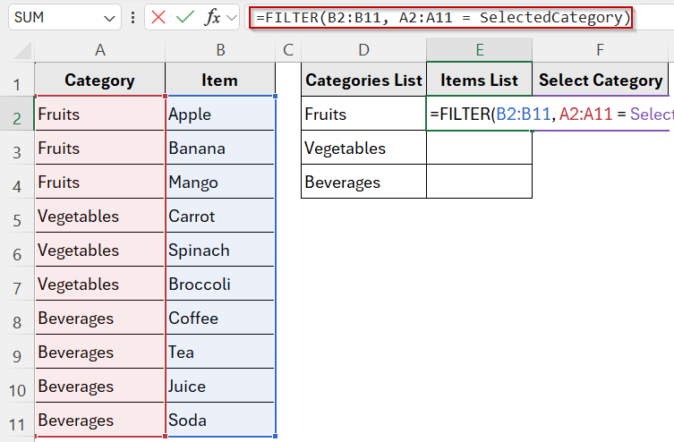
This will return only the items that match the selected category.
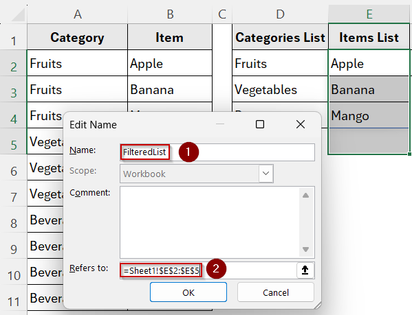
➤ Define a named range for the filtered list. Select E2 and go down to E10 (or as far as needed). Name it FilteredList by going to the Name Manager again.
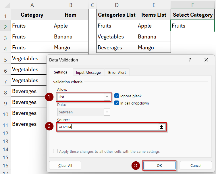
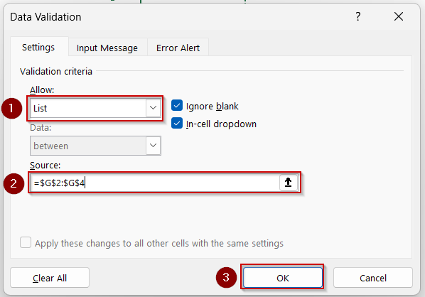
➤ Set up the first drop-down. In F2, go to Data >> Data Validation under Data Tools.
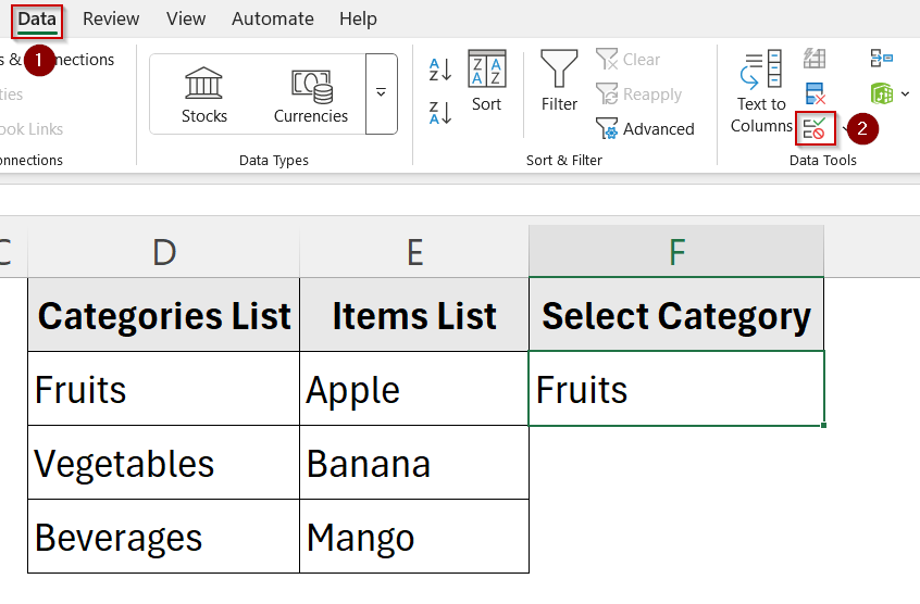
➤ Set Allow to List and point it to =D2:D4 (the unique categories) by typing in the Source box.
➤ Set up the second drop-down. In G2, go to Data >> Data Validation. Choose List under Allow and enter in Source box:
=FilteredList
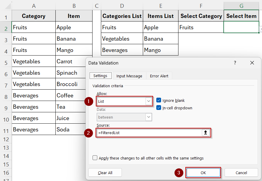
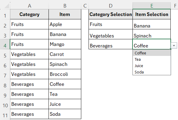
Now this drop-down will only show items that belong to the category selected in the first drop-down.
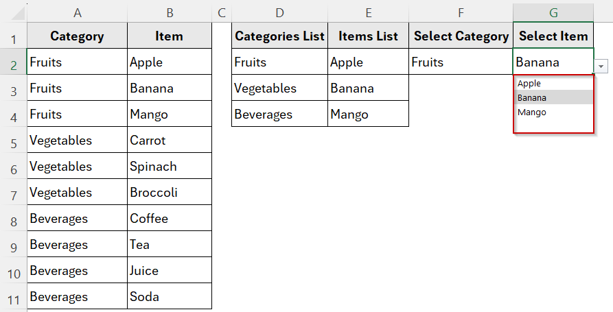
This method makes your drop-downs dynamic and responsive. Any time a user changes the category, the item list adjusts automatically based on the data.
Build Multiple Dependent Drop-Downs Across Rows
When working with tables or forms that require repeated user input, you may need multiple rows of dependent drop-down lists. For example, in an order entry sheet, each row might need a category and a matching item drop-down. This method shows how to apply dynamic dependent lists across rows so each pair works independently.
We will continue using the same 10-row dataset with “Category” in column A and “Item” in column B.
Steps:
➤ Create a unique list of categories. In cell H2, enter:
=UNIQUE(A2:A11)
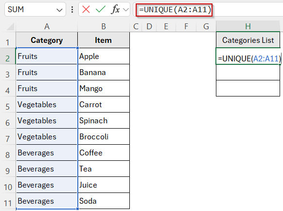
This generates a clean, non-repeating list of categories: Fruits, Vegetables, and Beverages.
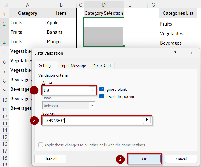
➤ Set up the category drop-downs. Select cells D2:D5. Go to Data >> Data Validation Data Tools.
➤ Choose List, and set the Source to:
=$H$2:$H$4
Now, each cell in column D provides a selectable list of categories.
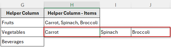
➤ Generate a filtered list of matching items. In cell I2, enter the formula:
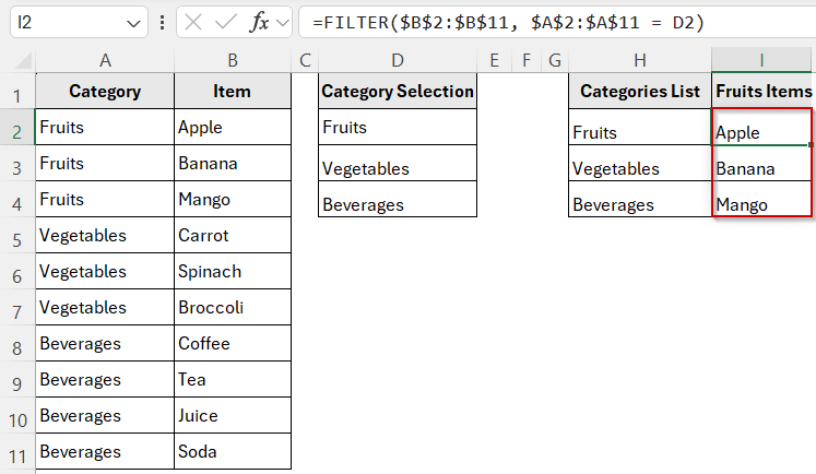
=FILTER($B$2:$B$11, $A$2:$A$11 = D2)
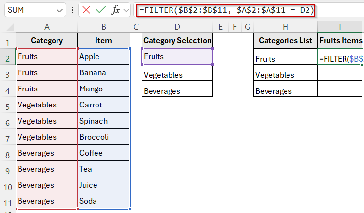
➤ Press Enter.
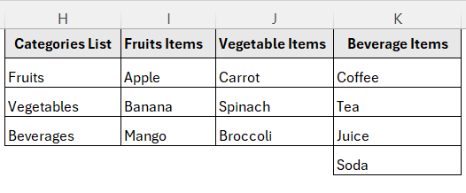
➤ Do the same for the rest of the categories. Enter the formula in J2 cell for Vegetables:
=FILTER($B$2:$B$11, $A$2:$A$11 = D3)
➤ Enter the formula in K2 cell for Beverages:
=FILTER($B$2:$B$11, $A$2:$A$11 = D4)
➤ The helper columns should look like this once setup is complete.
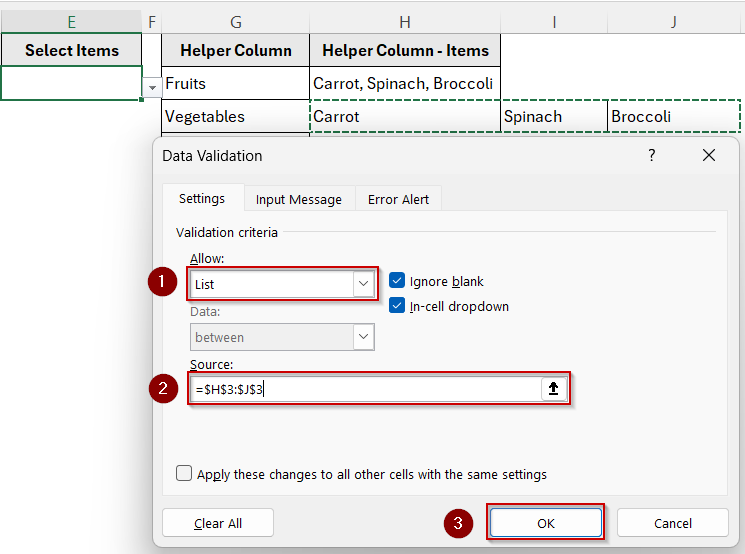
➤ Set up the dependent drop-downs. In E2 cell, go to Data >> Data Validation. Choose List, and in the Source box, enter: =I2#
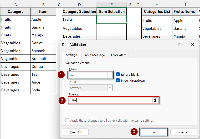
The hash symbol allows the drop-down to reference the entire dynamic spill range from column I.
➤ Repeat for each row. Apply similar validation to cell F3 through cell F5, using formulas like =J2#, =K2#, and so on, so each drop-down responds to its row’s selection.
This structure creates multiple independent pairs of dependent drop-downs that function row by row. It’s especially useful in structured forms where repeated input is required, such as product selectors, billing systems, or data entry templates.
Create an Expandable Drop-Down List That Updates Automatically
If your source data is likely to grow over time, it’s important to make your drop-down list dynamic so it expands as new values are added. Instead of manually updating the list range, you can set up an expandable drop-down that updates automatically whenever a new entry is added to the dataset.
We’ll use the same dataset in columns A and B. In this case, the focus will be on column B (items), and we’ll build a drop-down that reflects all items in real time, even as the list grows.
Steps:
➤ Create a dynamic named range. Go to the Formulas tab and click Name Manager >> New.
➤ In the dialog box, name it ItemList and refer it to:
=OFFSET(Sheet1!$B$2, 0, 0, COUNTA(Sheet1!$B$2:$B$100), 1)
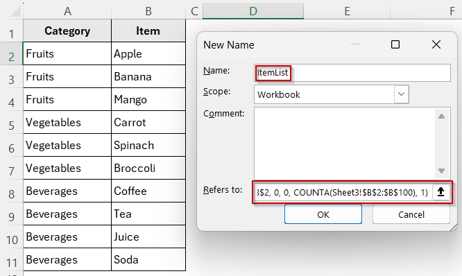
This defines a range that starts at cell B2 and automatically extends downward as more items are added.
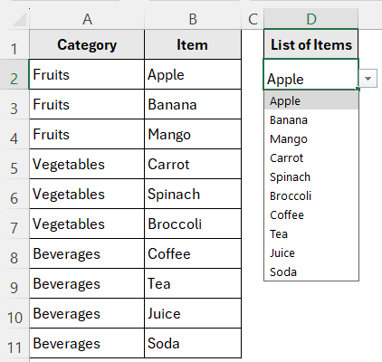
➤ Set up the drop-down list. Select cell D2 (or any cell where you want the drop-down).
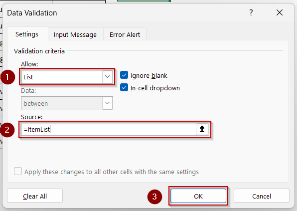
➤Go to Data >> Data Validation. Choose List, and in the source box, enter:
=ItemList
This connects your drop-down directly to the named range.
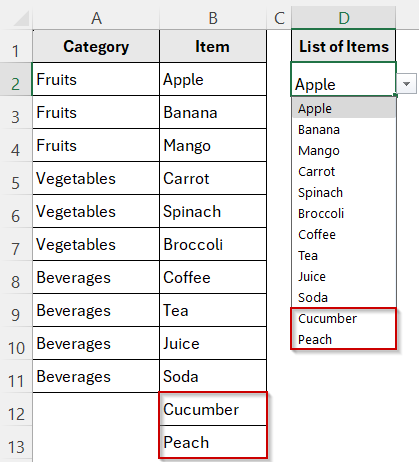
➤ Add new items to the dataset. Type a new item (e.g., “Peach” or “Cucumber“) into the next empty cell in column B. Then click the drop-down in D2 again, and you’ll see the new item automatically included.
➤ Use the drop-down across multiple cells. Copy the data validation in D2 to other cells (e.g., D4 or D6) to reuse the dynamic list anywhere in your worksheet.
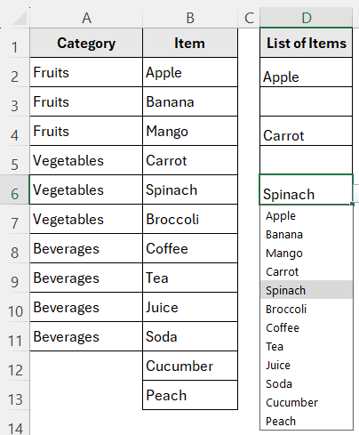
This approach is ideal for input sheets or dashboards where your list of options may grow over time. Once set up, the drop-down list remains in sync with your data, eliminating the need for manual updates.
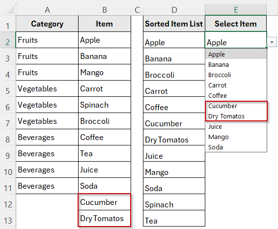
Sort a Drop-Down List Alphabetically Without Rearranging Your Data
By default, Excel drop-down lists display values in the order they appear in the source range. But if your data isn’t already sorted, this can make your drop-down look unorganized or harder to navigate. Luckily, you can create a drop-down list that appears alphabetically sorted, without having to actually sort your original dataset.
This method shows how to sort the list of items from column B alphabetically inside the drop-down, keeping your source data untouched.
Steps:
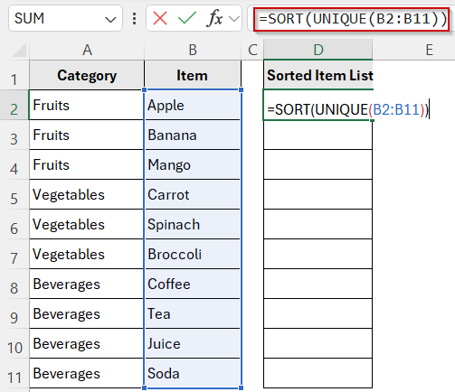
➤ Create a sorted version of your item list. Pick an empty helper column, such as D. In cell D2, enter the formula:
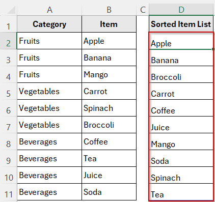
=SORT(UNIQUE(B2:B11))
This sorts the item names from column B in A–Z order while removing duplicates.
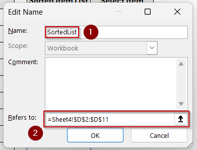
➤ Go to the Formulas tab, click Name Manager >> New, and create a named range and name it SortedList. Type in the Refers to box:
=$D$2:$D$11
This dynamically includes all sorted values from column D.
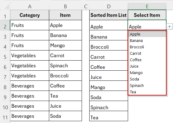
➤ Set up the drop-down. Choose the cell where you want your alphabetically sorted drop-down (e.g., E2). Go to Data >> Data Validation. Choose List, and enter this formula in the Source field:
=SortedList

➤ Test the drop-down. Click the drop-down in E2. You’ll see the items from column B displayed alphabetically, without modifying your original list.
➤ Anytime you add new items to column B, they’ll automatically appear in the drop-down in sorted order after being processed by the SORT formula.
This method is useful when your original data needs to stay as-is for reporting or other logic, but you still want a cleaner, more user-friendly drop-down experience.
Use Named Ranges with INDIRECT for Classic Dependent Drop-Downs
The INDIRECT function offers a reliable way to create dependent drop-down lists by referencing named ranges. This method has been used for years in Excel and still works well, especially when your data is relatively static and you need strong backward compatibility.
With this setup, the second drop-down list updates based on what a user selects in the first drop-down, using a direct reference to a named range.
Steps:
➤ Create named ranges for each category. From your dataset in columns A and B. Select B2:B4 (Fruits) and then go to Formulas >> Define Name. Name it Fruits
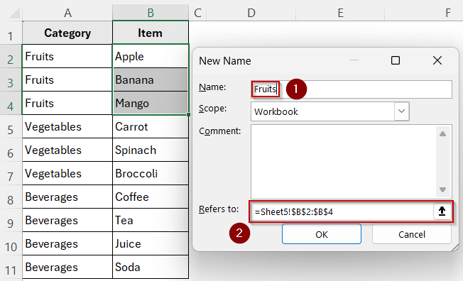
➤ Do the same for the rest of the categories.
These named ranges must exactly match the text values in column A.
➤ Set up the first drop-down. In cell D2, go to Data >> Data Validation, choose List, and set the source as:
=UNIQUE(A2:A11)
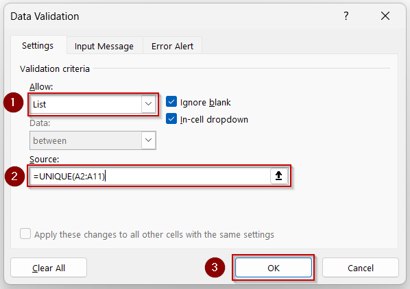
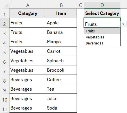
This drop-down will let users select a category like “Fruits” or “Beverages”.
➤ Set up the dependent drop-down using INDIRECT. In cell E2, go to Data >> Data Validation, choose List, and set the source as:
=INDIRECT(D2)
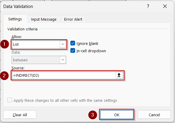
This uses the value selected in D2 to call the corresponding named range.
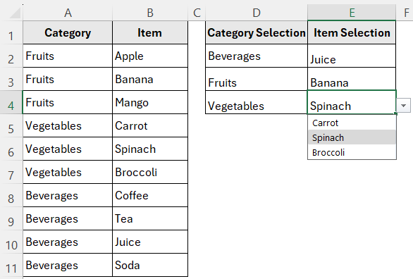
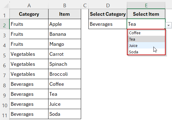
➤ Test your drop-downs. Try selecting “Vegetables” in F2. The second drop-down in G2 will now show only Carrot, Broccoli, and Spinach. Change it to “Beverages” to see Tea, Coffee, Juice, and Soda appear.
Create Dependent Drop-Downs with XLOOKUP
The XLOOKUP function offers a modern and flexible way to create dynamic dependent drop-down lists in Excel. Unlike traditional methods that rely on INDIRECT and named ranges, this approach uses a lookup formula to extract matching items from a dataset. It’s especially useful when you want to keep your data in one place without creating separate ranges for each category.
This method is ideal when working with structured datasets and looking for a formula-driven solution that is easier to maintain and update.
Steps:
➤ Create a helper column anywhere in the sheet, we are choosing G2. Enter this formula:
=UNIQUE(A2:A11)
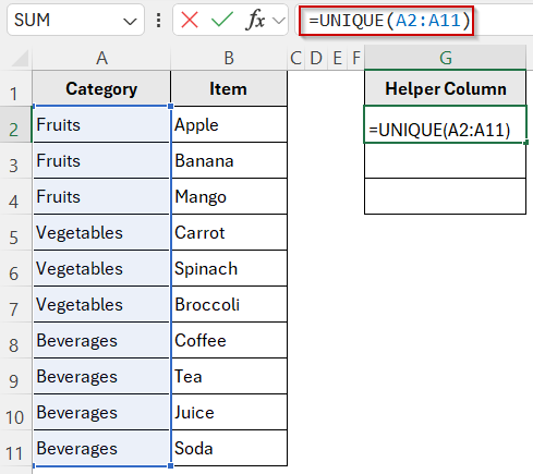
➤ Press Enter.
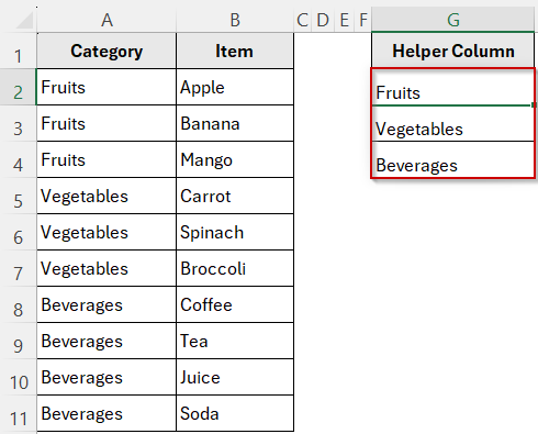
➤ Create the first drop-down list. In cell D2, go to Data >> Data Validation, choose List, and set the source as the helper column. In our case it’s G2:G4
This gives you a drop-down with category options: Fruits, Vegetables, and Beverages.
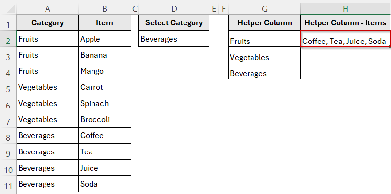
➤ Use XLOOKUP to extract matching items. In cell H2 (or any empty cell), enter the following formula:
=TEXTJOIN(“, “, TRUE, FILTER(B2:B11, A2:A11=D2))
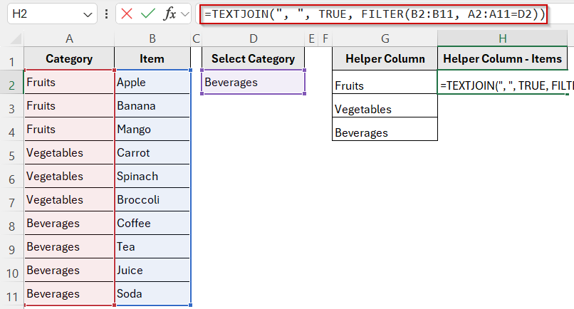
This pulls all items from column B that match the selected category in D2, and joins them into a comma-separated list.
➤ In cell H3, enter this formula:
=TEXTSPLIT(H2, “, “)

➤ Press Enter.
This splits the joined string from H2 back into a list Excel can use.
➤ In cell E2, go to Data >> Data Validation, choose List.. In the Source box, refer to the horizontal helper cells we created using TEXTSPLIT.
➤ Test the result. When you pick a category in F2, the drop-down in H2 will automatically update to show only the relevant items from that group.
Frequently Asked Questions
What is a dynamic dependent drop-down list in Excel?
A dynamic dependent drop-down list allows users to select values in one drop-down menu that determine the available options in a second drop-down. This setup updates automatically based on the selected value, making data entry more efficient and error-free.
Can I create dependent drop-down lists without using named ranges?
Yes, modern Excel functions like FILTER and XLOOKUP enable you to build dependent drop-downs without named ranges. These formulas pull matching data dynamically from your dataset, which makes your workbook easier to maintain.
Why do I get an error when using formulas like UNIQUE or TEXTSPLIT directly in Data Validation?
Excel’s Data Validation does not support dynamic array formulas directly in the Source field. To work around this, you must first spill the formula result into cells and then reference that cell range in your data validation list.
How can I create dependent drop-downs with more than two levels?
You can create multi-level dependent drop-downs by nesting dependent lists, where each drop-down’s options depend on the selection of the previous one. This requires using helper columns or dynamic formulas like FILTER combined with carefully structured datasets.
Wrapping Up
In this tutorial, we learned how to create dynamic dependent drop-down lists in Excel using various methods from traditional named ranges with INDIRECT function to modern approaches like FILTER, UNIQUE, and XLOOKUP. Each technique offers its own strengths depending on your version of Excel and how complex your data needs are. Feel free to download the practice file and share your feedback.