:Extracting data based on multiple criteria is a common need when working with large Excel tables. Whether you want to filter sales records by region and date, find employee details matching specific roles and departments, or compile lists from complex datasets, Excel offers several effective methods to get this done.
In this article, you will learn how to extract data from a table based on multiple criteria in Excel using functions and features like FILTER, Advanced Filter, SUMIFS, INDEX-MATCH, and more. These techniques work for both newer and older versions of Excel and help make your analysis faster, smarter, and more dynamic.
Steps to extract data from a table based on multiple criteria in Excel:
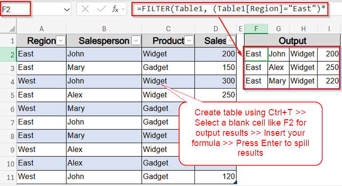
➤ Go to your table or create one using Ctrl + T and check your headers,
➤ Select the output start cell (e.g., F2).
➤ Enter formula:
=FILTER(Table1, (Table1[Region]=”East”)*(Table1[Product]=”Widget”), “No matching data”)
This filters rows where both Region is “East” AND Product is “Widget”.
➤ Press Enter to spill results automatically.
Apply the FILTER Function for Instant Multi-Criteria Results (Excel 365/2021)
The FILTER function is a dynamic array formula that returns an array of values meeting specified criteria. It’s the most straightforward and flexible way to extract data based on multiple conditions in the latest Excel versions.
Steps:
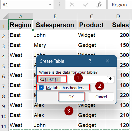
➤ Convert data into an Excel Table (Ctrl + T), making A2:D11 a structured reference. Make sure to check your headers and click OK.

➤ Select the output start cell (e.g., F2).
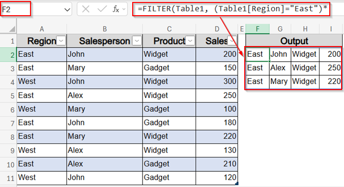
➤ Enter formula:
=FILTER(Table1, (Table1[Region]=”East”)*(Table1[Product]=”Widget”), “No matching data”)
This filters rows where both Region is “East” AND Product is “Widget”.
➤ Press Enter and results will spill automatically.
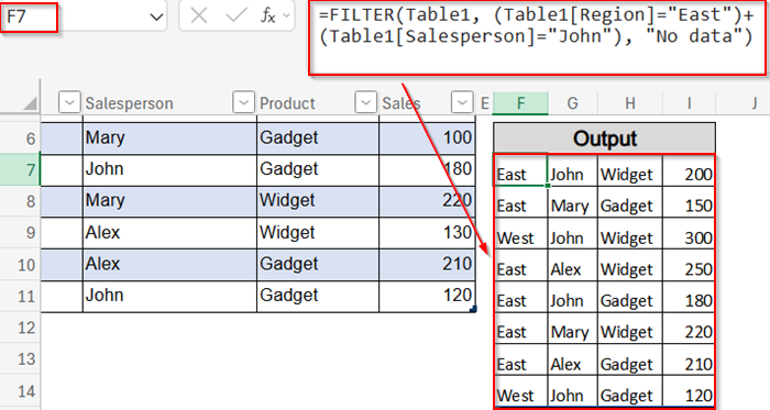
➤ You can adjust criteria by adding conditions. Insert this formula in F7 cell:
=FILTER(Table1, (Table1[Region]=”East”)+(Table1[Salesperson]=”John”), “No data”)
This filters rows where either Region is “East” OR Salesperson is “John”.
➤ Press Enter and results will spill automatically.
Here, formatting as a Table use ensures formulas reference column headers and automatically include new data. FILTER function also updates results automatically when the source data changes.
Set Up Advanced Filter Tool for Criteria-Based Extraction
If you’re using older Excel versions or want a no-formula solution, the Advanced Filter tool helps you extract rows based on AND/OR logic using a separate criteria range. It’s perfect for reusable, manual filtering tasks without dynamic formulas.
Steps:
➤ Arrange the dataset as a proper Table or consistent range.
➤ Convert data into an Excel Table (Ctrl + T), making A2:D11 a structured reference. Make sure to check your headers and click OK.

➤ Create a criteria range by setting headers (Region/Product) in F1:G1, and values (East/Widget) in F2:G2. These two rows (F1:G2) define your filter criteria.
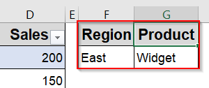
Excel reads this as “Only return rows where Region = East AND Product = Widget.”
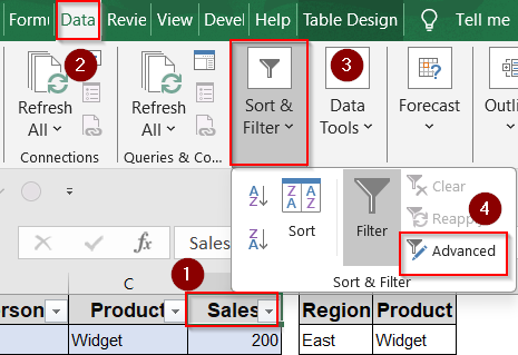
➤ Click anywhere inside your main table (A1:D11) such as D1 cell. Then, go to the Data tab >> Sort & Filter group >> Advanced.

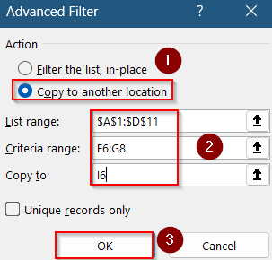
➤ Select “Copy to another location,” specify List range (A1:D11), Criteria range (F1:G2), and Copy to a blank area (J1).
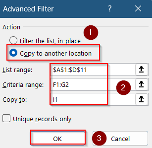
➤ Click OK and rows matching AND criteria are extracted.
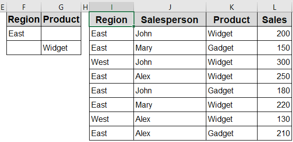
➤ To apply OR logic, list criteria on separate rows under the headers. Create a criteria range (e.g., in F6:G8).
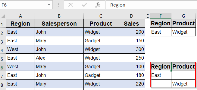
In this setup, cell F7 specifies that the Region must be “East” and cell G8 specifies that the Product must be “Widget,” so Excel treats this as an OR condition matching either criterion.
➤ Click anywhere inside your main table (A1:D11) such as D1 cell. Then, go to the Data tab >> Sort & Filter group >> Advanced.
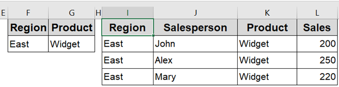
➤ Select “Copy to another location,” specify List range (A1:D11), Criteria range (F6:G8), and Copy to a blank area (I6).
➤ Click OK and your final output will appear instantly starting from I6 cell.
Advanced Filter allows for multiple criteria with AND logic by placing criteria in the same row and OR logic by placing criteria in multiple rows.
Use SUMIFS for Aggregate Results Based on Multiple Criteria
If your goal is to summarize values (like total sales for specific regions and products), SUMIFS function is ideal. This method doesn’t extract full rows but gives summed outputs based on multi-condition filtering which is perfect for dashboards or reports.
Steps:
➤ Convert data into an Excel Table (Ctrl + T), making A2:D11 a structured reference. Make sure to check your headers and click OK.

➤ In F2, enter:
=SUMIFS(Table1[Sales], Table1[Region], “East”, Table1[Product], “Widget”)
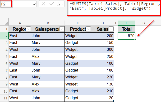
This returns the total sales where Region is “East” AND Product is “Widget” using structured Table references.
➤ Use wildcards or array constants for partial matches or OR logic, e.g., {“East”,”West”}
➤ For example, sum sales for all regions starting with “E” using this formula in F5 cell:
=SUMIFS(Table1[Sales], Table1[Region], “E*”)
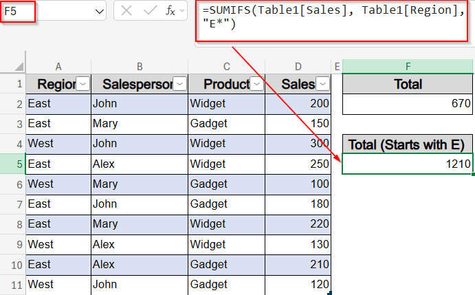
This sums the Sales where the Region starts with the letter “E” (e.g., East).
➤ Match products ending in “et” using this formula in F8 cell:
=SUMIFS(Table1[Sales], Table1[Product], “*et”)
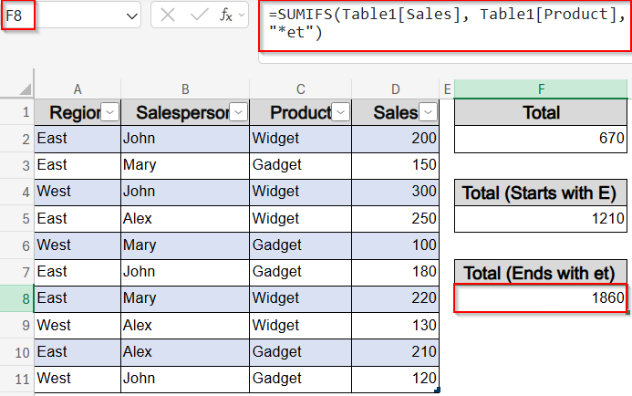
This sums Sales where the Product ends in “et” (e.g., Widget, Tablet).
Build Conditional Lookup Using INDEX & MATCH Array Formula
This method is best when you want to retrieve a single value (like sales or product) that matches two or more conditions. It combines logic-based matching with flexible cell referencing and works well even in Excel versions without FILTER.
Steps:
➤ Turn data into a Table to ensure dynamic reference and clarity. Press Ctrl + T >> Check your headers and click OK.

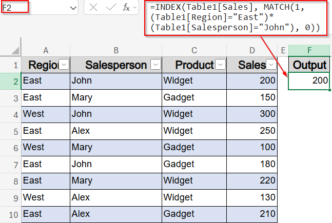
➤ In F2 (e.g., returns Sales):
This looks for the row where Region is “East” and Salesperson is “John“, then returns the corresponding Sales value.
➤ Press Enter in modern Excel; Ctrl + Shift + Enter in earlier versions.
Use XLOOKUP Function with Concatenated Helpers
XLOOKUP works well when paired with a helper column that joins multiple fields into a unique search key. This simplifies multi-criteria lookups into a single formula which is great for users comfortable with structured references and Excel 365 functionality.
Steps:
➤ Either keep range or use Table with extra helper column.
➤ Turn data into a Table to ensure dynamic reference and clarity. Press Ctrl + T >> Check your headers and click OK.

➤ Create helper column E (named “Key”) and enter this in E2 cell:
=[@Region] & “|” & [@Salesperson]
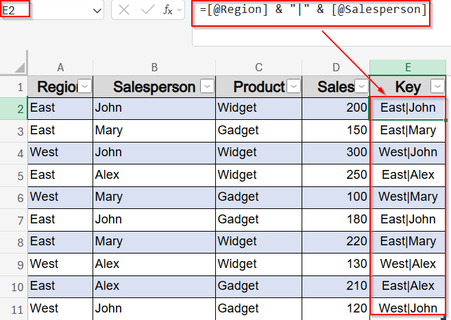
This creates a unique lookup key like “East|John” combining two fields.
➤ In G2, define Lookup Key (e.g., “East|John“).
➤ In H2, enter formula:
=XLOOKUP(G2, Table5[Key], Table5[Sales])
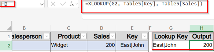
This searches the helper column for the exact key and returns the corresponding Sales in Output column.
Combine FILTER with SORT to Create Filtered Outputs
When you not only want to extract rows that meet certain criteria but also want them sorted, combining FILTER with SORT function gives you both. It’s especially useful when presenting results ranked by date, sales, or priority.
Steps:
➤ Turn data into a Table to ensure dynamic reference and clarity. Press Ctrl + T >> Check your headers and click OK.

➤ In F2 cell, enter this formula:
=SORT(FILTER(Table1, (Table1[Region]=”East”)*(Table1[Product]=”Widget”)), 4, -1)
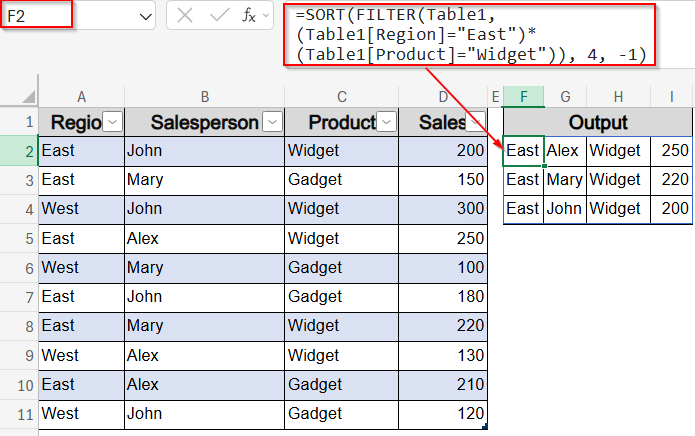
This filters rows matching both criteria, then sorts them by the 4th column (Sales) in descending order.
Apply Power Query to Filter Large Tables with Multiple Criteria
Power Query is ideal for users handling large datasets that need regular filtering and transformation. It enables repeatable, no-code logic to filter by multiple conditions and load the result into a new sheet or data model.
Steps:
➤ Turn data into a Table to ensure dynamic reference and clarity. Press Ctrl + T >> Check your headers and click OK.
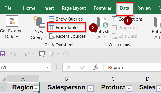
➤ Go to Data tab >> Under Get & Transform group, click From Table.
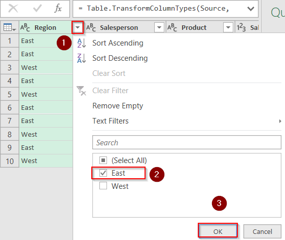
➤ In Power Query, apply filter steps for multiple criteria (e.g., Region = East, Product = Widget) using the small drop-down next to each column.
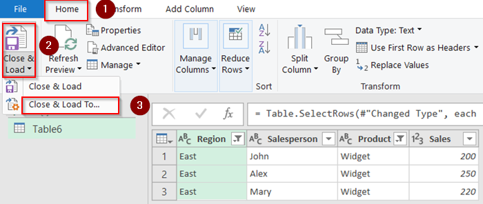
➤ Click Close & Load to from Home tab under Close & Load drop-down to return results as a new table.
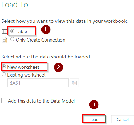
➤ Select Table and New worksheet. Then click Load on the pop-up window.
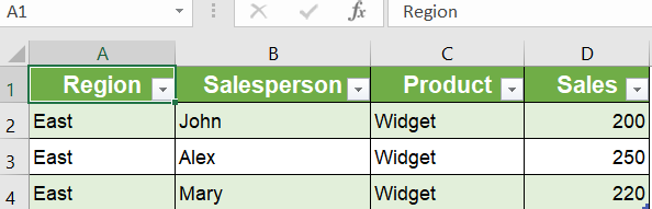
➤ Now your data will appear on a new worksheet as a new table maintaining your filters. Refresh anytime data changes pressing Alt + F5 without needing manual formula updates.
Frequently Asked Questions
How do I extract data based on two or more conditions in Excel?
Use the FILTER function in Excel 365 for dynamic results, or the Advanced Filter tool in older versions to extract rows that meet multiple column-based conditions without formulas.
Can I use SUMIFS to return full rows of data?
No, SUMIFS only returns a single aggregated result like total sales. To return entire matching rows, use functions like FILTER, INDEX-MATCH, or SUMPRODUCT depending on your Excel version.
Is Power Query better than formulas for filtering?
Yes, Power Query is a great option for large datasets. It allows repeatable filtering steps, automatic updates, and better performance compared to formulas, especially when filters need frequent adjustment.
Wrapping Up
In this tutorial, we learned how to extract data from a table based on multiple criteria in Excel using a range of methods suited to different versions and tasks. Whether you’re working with dynamic formulas, helper columns, or Power Query transformations, Excel gives you all the tools to filter your data precisely. Feel free to download the practice file and share your feedback.