
Repeated entries in Excel can affect your report and analysis if the duplicate data is not dealt with properly. It does not matter whether you are working with customer details, financial reports, or inventory data. By detecting the data, you can keep your data clean and reliable. One of the most efficient ways to do that is to use the VLOOKUP function of Excel. No matter if you’re working with single or multiple worksheets, this function can easily find those.
To find the duplicate values in Excel you can follow the below steps-
➤ Make sure your datasets have two columns to compare duplicate values.
➤ In the empty cell beside your column, write the formula for VLOOKUP.
➤ Enter the following formula and press Enter –
=IF(NOT(ISNA(VLOOKUP(A2, C:C, 1, FALSE))), “Duplicate”, “Not Duplicate”)
Here, the cells in the A column are compared with the values of the C column.
➤ Drag the cells down for Fill Handle and apply it to the rest of the cells.
➤ The cells will display the word ‘Duplicate’ if the value is repeated in both columns, and ‘Not Duplicate’ will be visible for unique values.
In this article, we will dive into the various aspects of the VLOOKUP function, what it is, and how it works. We will see how to find the duplicate values in Excel using the VLOOKUP in single and multiple worksheets across different files. Along with solving the common errors, we tried to help walk through each method step-by–step with proper understanding.
What is the VLOOKUP Function in Excel and What Does it Do?
VLOOKUP mainly stands for Vertical LookUp and is a powerful function of Excel. Being one of the widely used tools in Excel, it has multiple uses. It can retrieve data from a structured list, compare values across tables, and match data from different columns in order to find duplicates.
In case of finding duplicate values, VLOOKUP comes in handy. It searches the value in the first column of a range and compares it with all the cells of the other specified column.
VLOOKUP has the following formula syntax-
=VLOOKUP(lookup_value, table_array, col_index_num, [range_lookup])
![]()
Here, the lookup_value is the cell number that contains the value to search for. The table_array is the range of the cells that you want to search. Lastly, the col_index_num is the column you want to return a value if the data match, and the range_lookup is the value you want to display (such as true for duplicates and false for unique ones)
Identifying Duplicates Within the Same Sheet
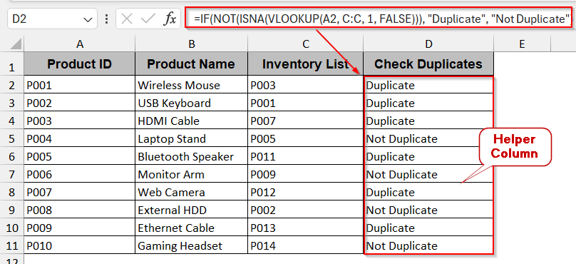
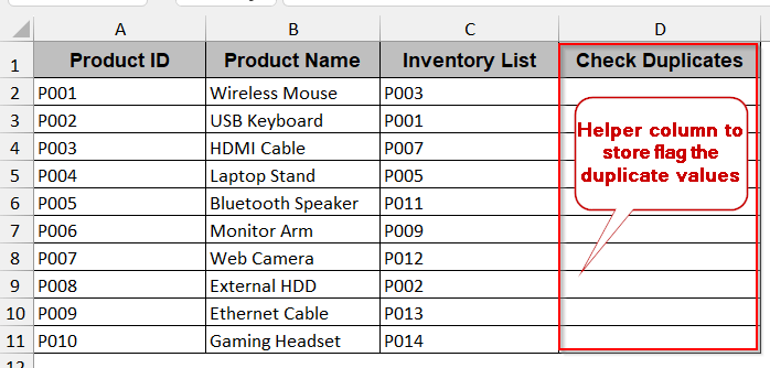
For finding the duplicates between the data of two columns in the same sheet, VLOOKUP can be most helpful. In this example below, we have a list of Product IDs in column A and a separate column of Inventory List in Column C. Our task is to find out if the product IDs of column A are also present in column C as inventory list due to duplication. We will flag those values as ‘Duplicate in the cell beside each value.
Steps:
➤ Select the cell beside the column you want to check. For a better presentation, named in Check Duplicate.
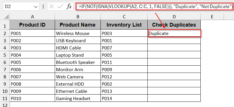
➤ In the first row of the cell, write the formula of VLOOKUP –
=IF(NOT(ISNA(VLOOKUP(A2, C:C, 1, FALSE))), “Duplicate”, “Not Duplicate”)
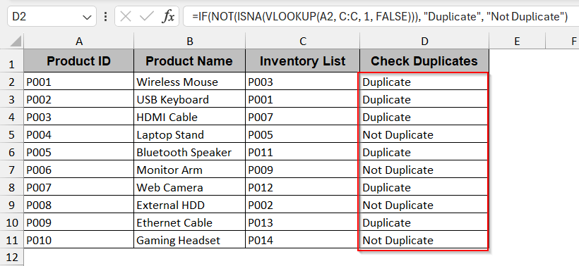
➤ Press Enter to apply the formula in the cell. If an exact duplicate is found, the cell will display ‘Duplicate’ and otherwise, it will show ‘Not Duplicate’.
➤ Use Fill Handle to drag the cells and apply the same formula to the rest of the cells.
Note:
➨ If you want to keep the unique values as blank, modify the formula as pass nothing inside the last quotation marks.
➨ This method does not highlight the duplicate values like conditional formatting. It only flags them with text.
Finding Duplicates Between Two Worksheets Using VLOOKUP
The first method is more idealistic than realistic. In a real-world scenario, you might often need to find duplicates across multiple sheets of the same file. Luckily, VLOOKUP also has the functionality to check between the worksheets and find duplicate values.
To illustrate, we will be having two sheets in one Excel file, one named Sales and another named Inventory. The Sales sheet consists of the product IDs and the product names. On the other hand, the Inventory sheet contains only the ID of the inventory list. Again, we will check if the product IDs have duplicate values in the inventory list.
Steps:
➤ Go to the sheet in which you want to flag the cells with duplicate values.
➤ In the cell beside the desired column, create a new column with the name Check Duplicate.
➤ Write the following formula in the first cell of the column –
=IF(NOT(ISNA(VLOOKUP(A2, Inventory!A:A, 1, FALSE))), “Duplicate”, “Not Duplicate”)
Here, the A2 is the first cell of the column Product IDs from the first sheet, and the A:A is the range of the cells of the second sheet of the Inventory List.
➤ Press Enter to generate the formula for the specific cell.
➤ Drag the cells and Fill Handle to apply the same formula to the rest of the cells.
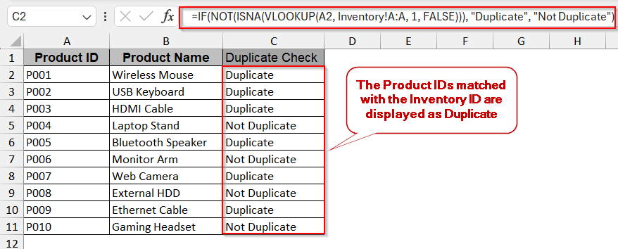
➤ Any value in the first sheet of the column will be displayed as ‘Duplicate’ if it is present in the second sheet too.
Note:
➨ Replace the VLOOKUP formula with your first column cell (A2), the range of the selected column (A:A), and the name of the other sheet (here it is Inventory).
➨ This formula is specifically curated for multiple sheets. Thus, it won’t be useful otherwise.
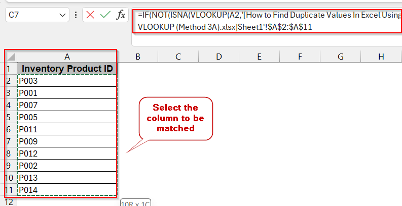
Duplicate Identification Across Different Excel Files Using VLOOKUP
VLOOKUP also gives you the flexibility to check the duplicates within different Excel files. This feature helps a lot when you need to deal with large, diverse data for different departments.
Here, again, we are considering that we have two Excel files named Sales and Inventory. The Sales sheet consists of the product IDs and the product names. These product IDs have to be checked with the inventory IDs from the Inventory sheet.
Steps:
➤ Open both of the Excel files simultaneously.
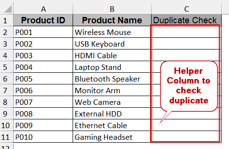
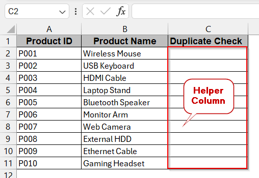
➤ Create a helper column named Duplicate Check to store the values to determine if it is duplicated or not. You can only create one column in one of the workbooks.
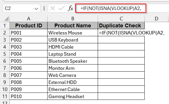
➤ In the first cell of that column, first write the VLOOKUP formula –
=IF(NOT(ISNA(VLOOKUP(A2,
where, A2 is the first cell of the column that needs to be matched.
➤ Now, go to the next file and select the entire column you want to check. This will automatically generate the next part of the formula after A2.
‘[How to Find Duplicate Values In Excel Using VLOOKUP (Method 3A.xlsx]Sheet1’!$A:$A
where A:A is the range of the cells in the other Excel file.
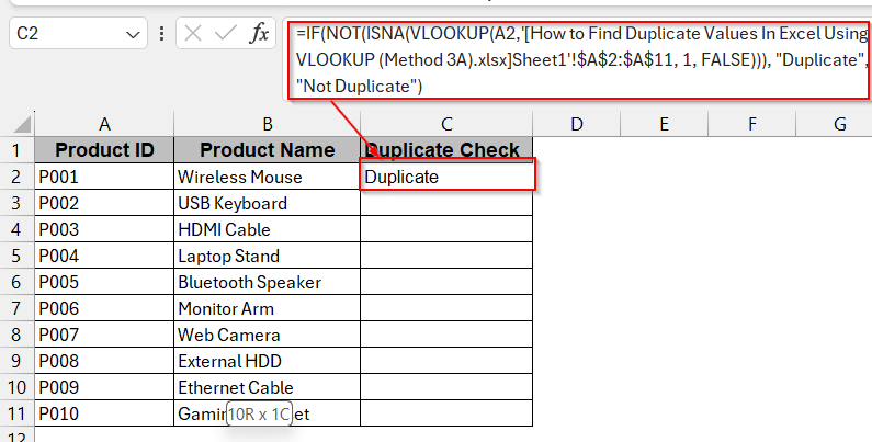
➤ Complete the rest of the formula in a similar pattern to the previous methods. The entire formula will look like this.
=IF(NOT(ISNA(VLOOKUP(A2, ‘[How to Find Duplicate Values In Excel Using VLOOKUP (Method 3A).xlsx]Sheet1’!$A:$A, 1, FALSE))), “Duplicate”, “Not Duplicate”)
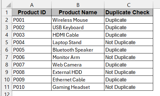
➤ Press Enter, and it will display “Duplicate” or “Not Duplicate” depending on your values.
➤ Drag the cells to apply the Fill Handle to generate the same formula for the rest of the columns.
Note:
➨ Replace the ‘Inventory’ and the sheet number according to your workbook
➨ Make sure to open both files to avoid #REF errors.
➨ It is recommended to keep both the workbooks in the same folder.
Why VLOOKUP Isn’t Always Enough for Handling Duplicates
While VLOOKUP is a powerful Excel tool specifically curated to find and check the matched data, it might not always be the perfect one. It has several minor to major limitations when trying to identify duplicate values. Understanding these constraints is crucial to know when you should use VLOOKUP or move to other tools.
- Returns the first match: VLOOKUP can’t return multiple results for a duplicate value; only the first one is processed.
- Lacks flexibility in Duplicate Counting: No special formula is available in VLOOKUP that will help to count how many duplicate values are found.
- Can’t work with the columns left: One of the major drawbacks is that it can’t check your required column against the left columns. It can only check the duplicates with the right-hand side columns beside your designated one.
- Formatting Issues: With extra spaces, mismatched data types, and hidden characters, VLOOKUP might fail to find the duplicate value.
- Performance Issues: When working with large datasets, repeated use of the VLOOKUP formula can slow down the entire performance flow of the file.
Frequently Asked Questions
Why does Excel not recognize duplicates correctly when using VLOOKUP?
VLOOKUP can fail to recognize duplicates correctly when you have more than one duplication of the same value. As it only checks the first one, it might not work for the rest. Except that there might be formatting issues like wrong data types and extra spaces.
How do I filter or highlight duplicates in Excel?
To filter or highlight duplicates in Excel, select the entire column or row that you want to apply the rules to. Click on Conditional Formatting in the Home Tab. From the dropdown menu, choose the Highlight Cell Rules and then Duplicate Values.
What do I do if VLOOKUP returns incorrect data from duplicate values?
If VLOOKUP returns incorrect data, you have to use a different Excel function. The most common ones from them are INDEX and MATCH, Filter, and XLOOKUP.
Why am I seeing #N/A even though the value looks duplicated?
The #NA in the duplicated value means Excel failed to check duplicate values using VLOOKUP. These usually happen to the mismatched data types, extra leading and trailing spaces, hidden characters, etc.
Can VLOOKUP find duplicates across multiple sheets or workbooks?
VLOOKUP has the function to find duplicates across multiple sheets and workbooks. You just need to modify the formula structure a bit and mention the names of the sheets.
Concluding Words
VLOOKUP is the widely used and practical solution when you need to find duplicate values. Whether you need to use it for a single or multiple sheets and even for different Excel files, VLOOKUP is the first function we look up to. The methods for executing these are quite easy and doable if you follow the steps properly.
Go through our workbooks and examples and understand for what cases your data needs VLOOKUP. Share your feedback and help us make your experience even better.