Data analysis often requires us to parse texts in different ways. You might need to clean some data, extract some words, or validate a string. As there is no direct function in excel to find the last occurrence of a character in a string, you need to get creative. In this article, we will learn five ways to find last occurrence of characters in string in excel.
➤ In a helper cell, write this formula:
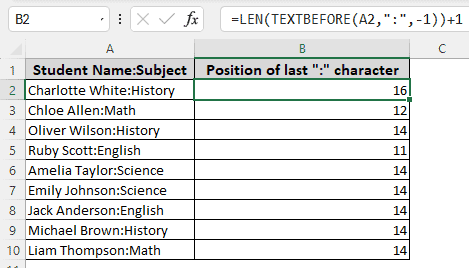
=LEN(TEXTBEFORE(A2,”:”,-1))+1
➤ Replace A2 with your input cell, “:” with your desired character, and Press Enter.

That was one way of doing that. However, for flexibility, you might want to learn some more ways to do that. In this article, we will present a total of five methods for doing the job. Therefore, consider reading the whole article to understand the procedures and explanations.
Finding Last Occurrence of Character Using the LEN-TEXTBEFORE Functions
In this sample, we have a dataset containing some records of students, including their subject names. The administration wants to parse these records programmatically later. The subject names and the student names are separated using a colon (:). In order to separate those, we need to find the position of the colon.
This formula is probably the smallest one in the whole article. We are going to use only two functions and find the exact position of the desired character. The steps to be followed are below:
➤ Select the cell where you want to get the last occurrence location.
➤ Enter this formula:
=LEN(TEXTBEFORE(A2,”:”,-1))+1
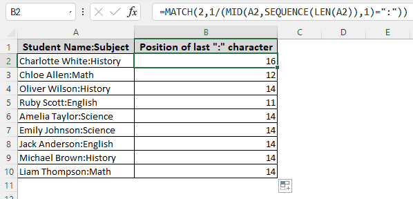
Using a Combination of MATCH-MID-SEQUENCE-LEN Function
We are going to use a formula that is a bit more complex than before. There will be four functions in the work today, and we will learn how those work together for our desired output.
➤ Just like before, select a cell, and put this formula in:
=MATCH(2,1/(MID(A2,SEQUENCE(LEN(A2)),1)=”:”))
➤ Press Enter after replacing A2 with your string/input cell, and “:” with your character.
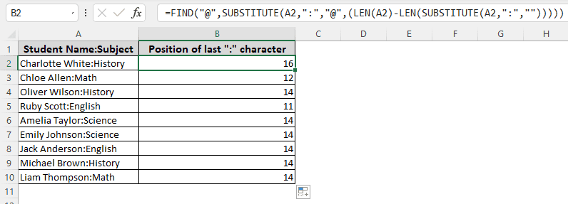
Applying Another Formula with FIND-SUBSTITUTE-LEN Functions
This method is something we will not recommend you use for every case. The functions replace the desired character with something else to do the job. However, if you already have the replacement character in the string, the formula fails miserably. Only use this method if you have to.
➤ Paste this formula in the helper cell:
=FIND(“@”,SUBSTITUTE(A2,”:”,”@”,(LEN(A2)-LEN(SUBSTITUTE(A2,”:”,””)))))
➤ Do not forget to replace A2 with your input cell and “:” with your character.
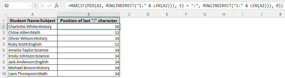
Using MAX-IF-MID-ROW-INDIRECT-LEN Functions
This is going to be the largest formula in this whole article. If you want to understand the formula, read the explanation part carefully. If you don’t, just replace the input cell and the desired character, and you will be good to go.
➤ Place this function in the output cell:
=MAX(IF(MID(A2, ROW(INDIRECT(“1:” & LEN(A2))), 1) = “:”, ROW(INDIRECT(“1:” & LEN(A2))), 0))
➤ Press Enter.
Running VBA Code
Tired of all these functions? We are now making things a bit more interesting. We are going to use some visual basic coding to accomplish the job. Follow the steps below:
➤ Press Alt+F11 to open the code editor.
➤ From the top menubar, go to Insert > Module.
➤ Write this code in the window:
Public Function GetLastCharacterPosition(inputText As String, targetChar As String) As Integer
Dim position As Integer
position = -1
Dim index As Integer
For index = Len(inputText) To 1 Step -1
If Mid(inputText, index, 1) = targetChar Then
position = index
Exit For
End If
Next index
GetLastCharacterPosition = position
End Function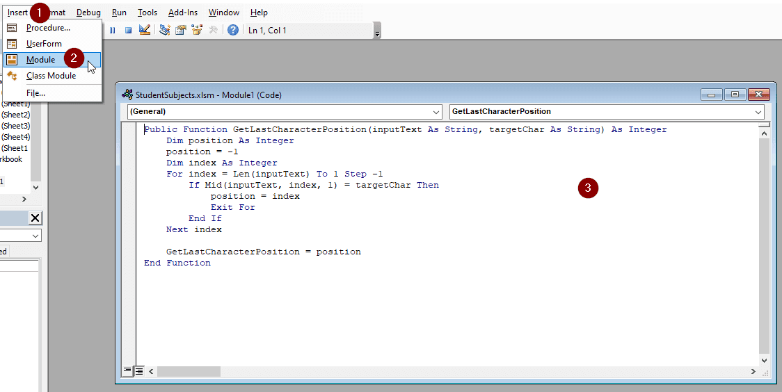
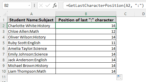
➤ Go back to the spreadsheet, and write this code:
=GetLastCharacterPosition(A2, “:”)
➤ Replace A2 with your input cell and “:” with your desired character.
➤ Press Enter.
Frequently Asked Questions
How to extract last 5 characters in Excel?
Use this formula:
=RIGHT(A1,5)
Replace A1 with your input cell.
How to get first 10 characters from string in Excel?
Type this formula:
=LEFT(A1,10)
Here, A1 is the input cell.
What is the value of the last character in a string?
It is the length of the string minus 1. In excel you can put this:
=LEN(A1) – 1
A1 will be the input string cell.
How to extract middle 4 characters in Excel?
This formula should suffice:
=MID(A1, LEN(A1)/2 -2 ,4)
Here, A1 is the input cell. The MID function takes the input cell, the point where it should start extracting, which is determined using the LEN function, and how many characters it needs to extract.
How do I separate text in Excel?
From the menu of excel, go to Data>Text to Columns. Then the Convert Text to Columns wizard will guide you through the process of separating text into different columns.
Wrapping Up
In this article, we have learned five ways to find the last occurrence of a character in a string using excel. The practice file contains all of the methods used in this article. Feel free to use the file and leave a suggestion below for us on how we can improve.