When we work with large datasets, sometimes we need to find a specific text within a range and then return its cell reference. It is a common practice. For example, this is useful in inventory tracking, employee databases, or maybe any searchable list where you need to have the exact location of a value rather than just the value itself. Another example is when users want to dynamically reference a cell for automation, lookups, or conditional formatting.
To find text in range and return cell reference, follow these steps:
➤ Use the MATCH function to find the position of the text in the range.
➤ Wrap the result in INDEX to return the corresponding cell.
➤ Use the CELL(“address”, …) function to return the cell reference.

Here, in this article, we’ll look into multiple methods to find text in a range and return the cell reference using Excel formulas like INDEX, MATCH, and CELL. We’ll also answer frequently asked questions and analyze use case examples.
Combine CELL, INDEX & MATCH Functions to Find Text and Return Cell Address
We will use a combination of MATCH, INDEX, and CELL. It will search for a specific value (text) within a range and return the cell address where that value is located. Open your worksheet or navigate to our demo worksheet (Sheet 1).
Steps:
➤ On cell D2 & E2 write Cell Position and Cell Address for reference. We will retrieve cell position of any input data in D3 cell and cell address in E3 cell.
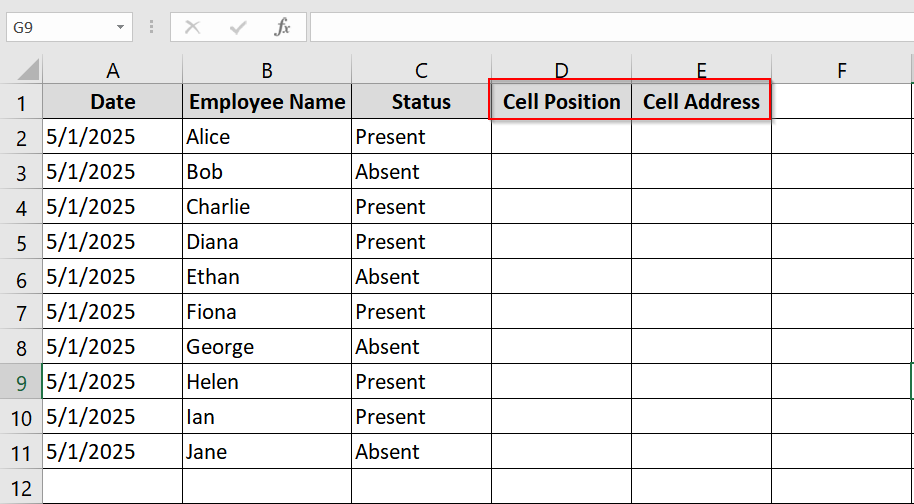
➤ Determine which column you’ll be searching. For example Column B for employee names). Highlight or note the range: here, it’s B2:B11.
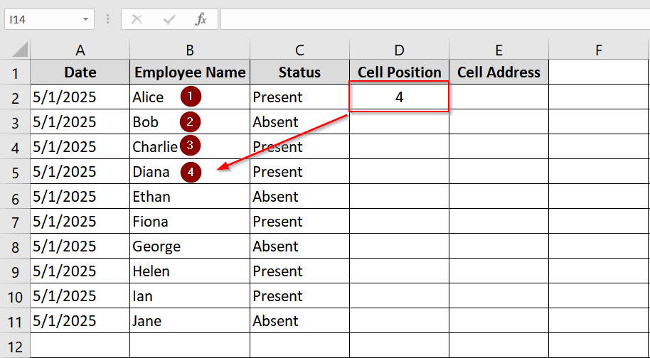
➤ Type the MATCH function in cell D3 to get the position of the desired name in the range. If we want to find the cell position for Diana the function will be like-
=MATCH(“Diana”, B2:B11, 0)
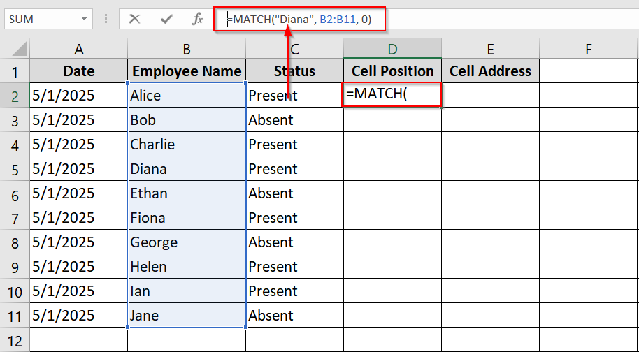
➤ This returns 4 because “Diana” is the 4th item in the B2:B11 range.
➤ Use CELL to Get the Address of That Cell
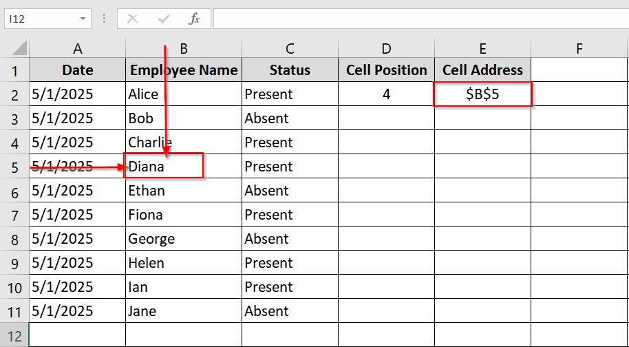
Wrap the INDEX formula inside the CELL function. If we want to find the cell reference or cell address for Diana it the formula in E3 will be-
=CELL(“address”, INDEX(B2:B11, MATCH(“Diana”, B2:B11, 0)))

➤It returns the address of the cell as a string: $B$5.
Notes:
➧ This method returns the address of the first occurrence of the text. If the text appears multiple times, only the first match will be considered.
➧ The range must be one dimensional (a single row or a single column).
Dynamically Find the Cell Reference of Any Text using CELL, INDEX & MATCH Function
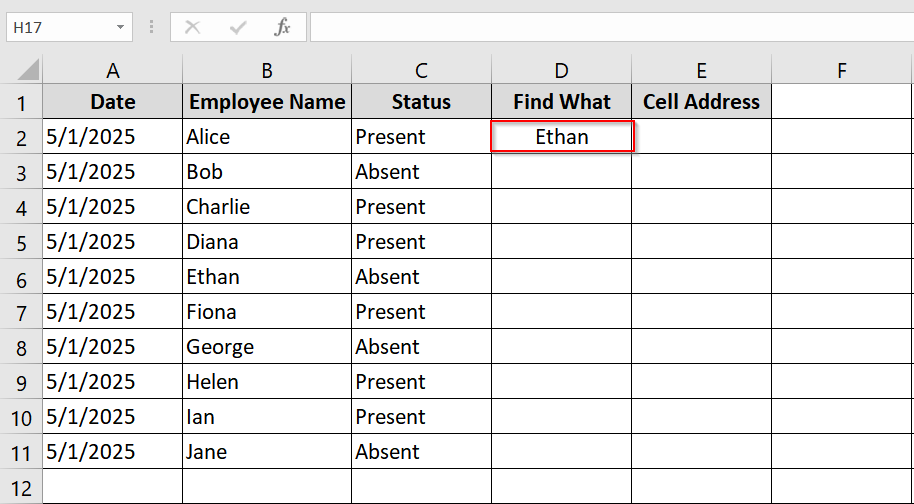
This method will locate the cell reference of an employee’s name in a dataset. This process is dynamic. Once the function is in place, you can just type anything in a cell and get the cell reference in another cell. For example, if you need to find where “Ethan” appears in the list, this method gives you the exact cell address.
Steps:
➤ Open your Excel worksheet.
On cell D2 & E2 write Find What and Cell Address for reference. We will write what we want to find in D3 cell and will automatically get cell reference in E3 cell
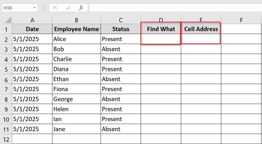
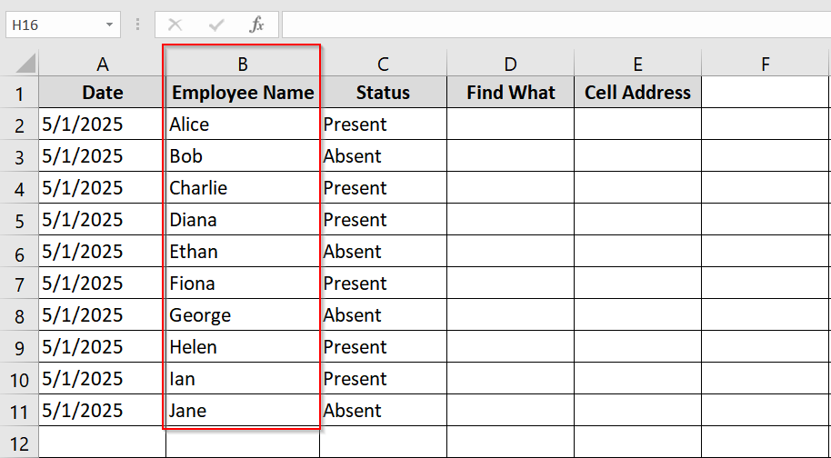
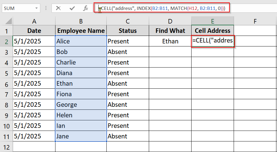
➤ Decide on which range you will work on. In this example, Employee names are in cells B2 to B11. That is our search range.
➤ Enter the Name to Search in cell D3
➤ Write this formula in E3 to return the address.:
=CELL(“address”, INDEX(B2:B11, MATCH(E1, B2:B11, 0)))
➤ After entering the formula, press Enter. You’ll now see a result like: $B$6
This is the exact cell where “Ethan” is found.
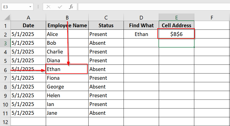
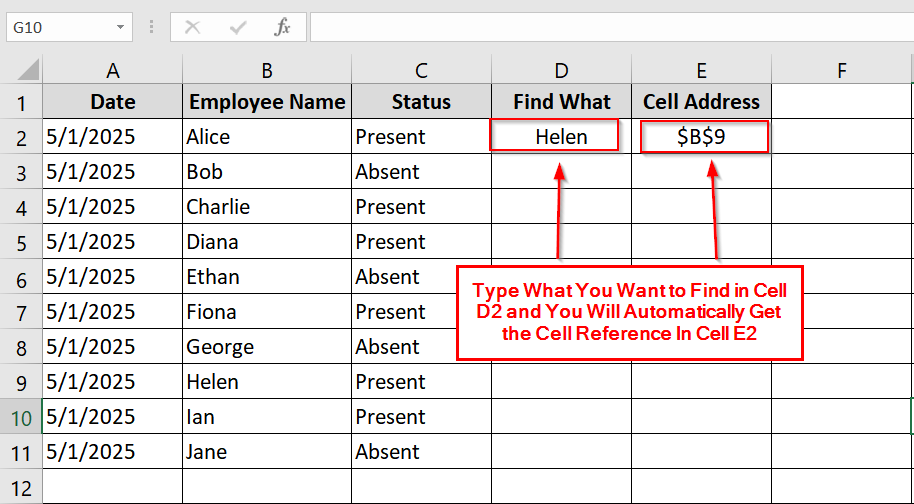
➤ Now you can write any text in the D3 cell and the E3 cell will return with its cell reference. It’s now dynamic. You won’t have to type a formula each time.
Notes:
➧ This method is case insensitive. “ethan” and “Ethan” will both work.
➧ If the name is not found, the formula will return #N/A.
➧ It only finds the first match. If the name appears more than once then it will return the address of the first one.
Implementing CELL + INDEX + MATCH for Horizontal Search
For this method, we will Implement CELL + INDEX + MATCH for Horizontal Search (Row wise Text Search). This method is used to find the cell address of a value that is located horizontally across a row.
Here we will find the address of the column labeled “Jul“. So our search text is “Jul“.
Steps:
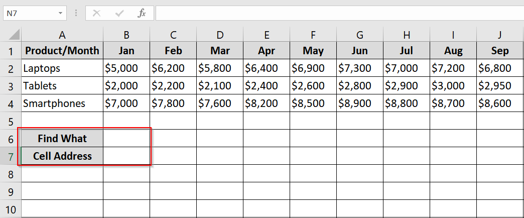
➤ Open up your excel worksheet where horizontal search is needed. On cell A6 & A7 write Find What and Cell Address for reference. We will type what we want to find in B6 cell and cell address will automatically appear in B7 cell
➤ Choose the row where you want to find your data. In this case B2:J2
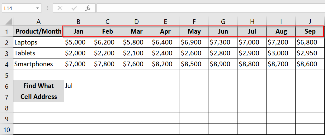
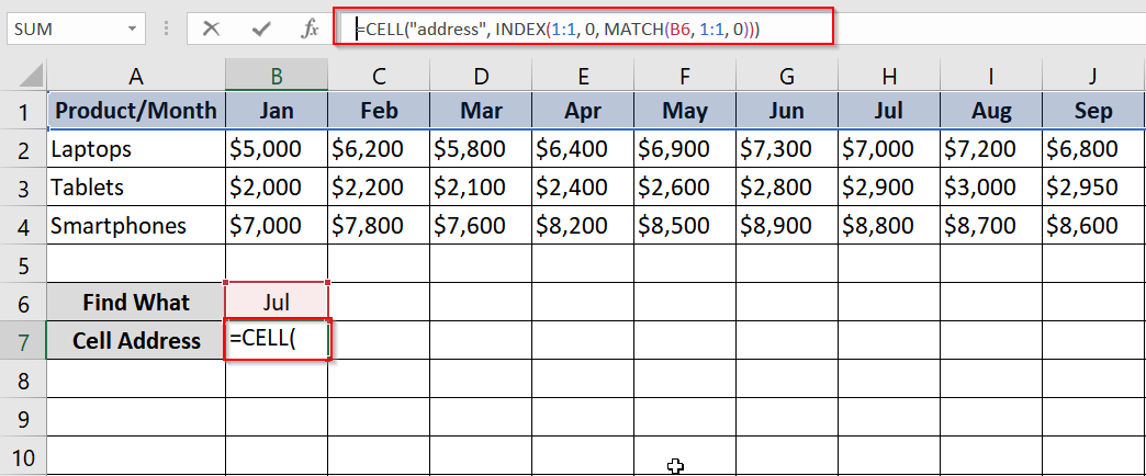
➤ Write the name Jul in B6 and formula in B7
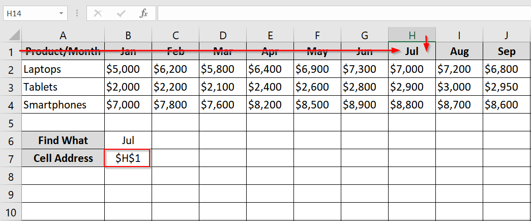
=CELL(“address”, INDEX(1:1, 0, MATCH(“Jul”, 1:1, 0)))
➤ This returns $G$1 (address where “Jul” is found).
Notes:
➧ The formula returns the cell address as text, not the value.
➧ If the value is not found, the formula will return a #N/A
Use MATCH, INDEX & ADDRESS Functions Separately to Return Values or Cell Addresses
Instead of only finding the position of a value using MATCH, you can combine it with INDEX to return the actual value, or with ADDRESS to return the cell reference where it appears.
Steps:
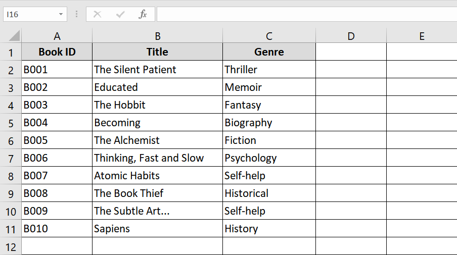
➤ Set up a clean vertical list of data. For this example, book titles are in range B2:B11.
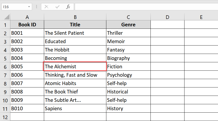
➤ Choose the keyword to look for. It can be typed directly or referenced from another cell.
Example: “The Alchemist” or a cell with the value.
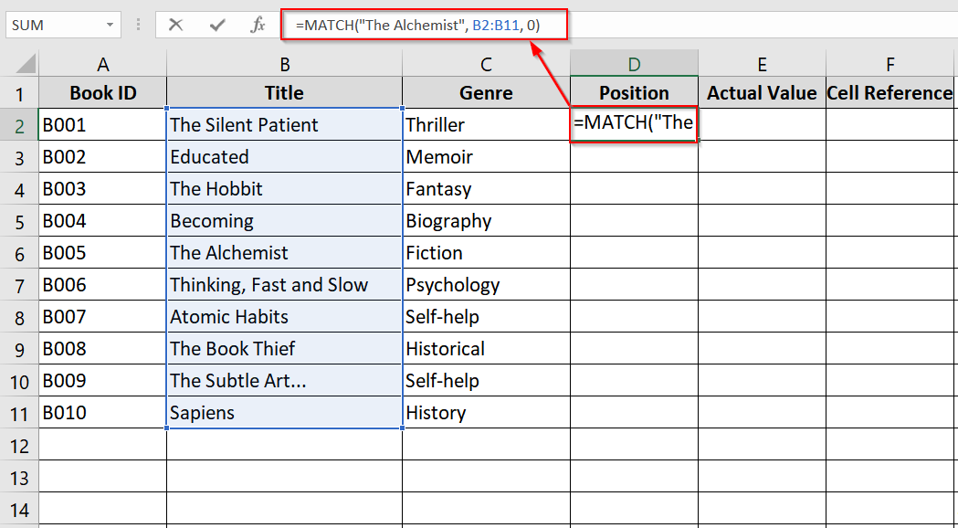
➤ Use MATCH to get a position. Find where the value appears within the list:
=MATCH(“The Alchemist”, B2:B11, 0)
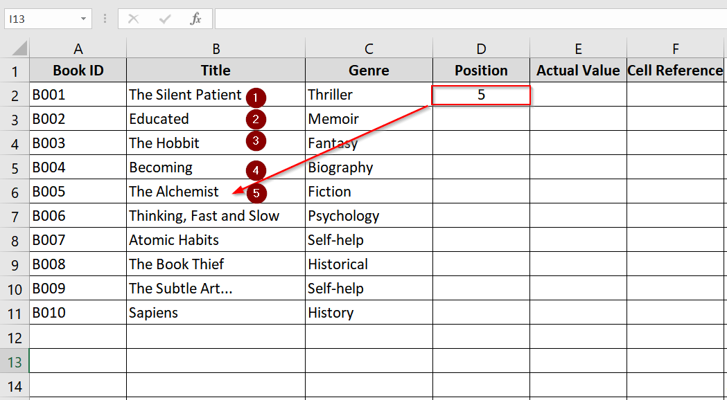
➤ This returns 5 if it’s the 5th item in the list.
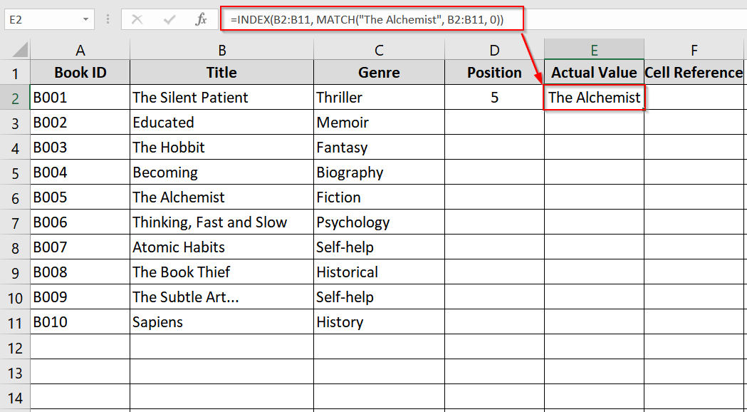
➤ To return the actual value using INDEX + MATCH, combine INDEX with MATCH:
=INDEX(B2:B11, MATCH(“The Alchemist”, B2:B11, 0))
This returns the value “The Alchemist”.
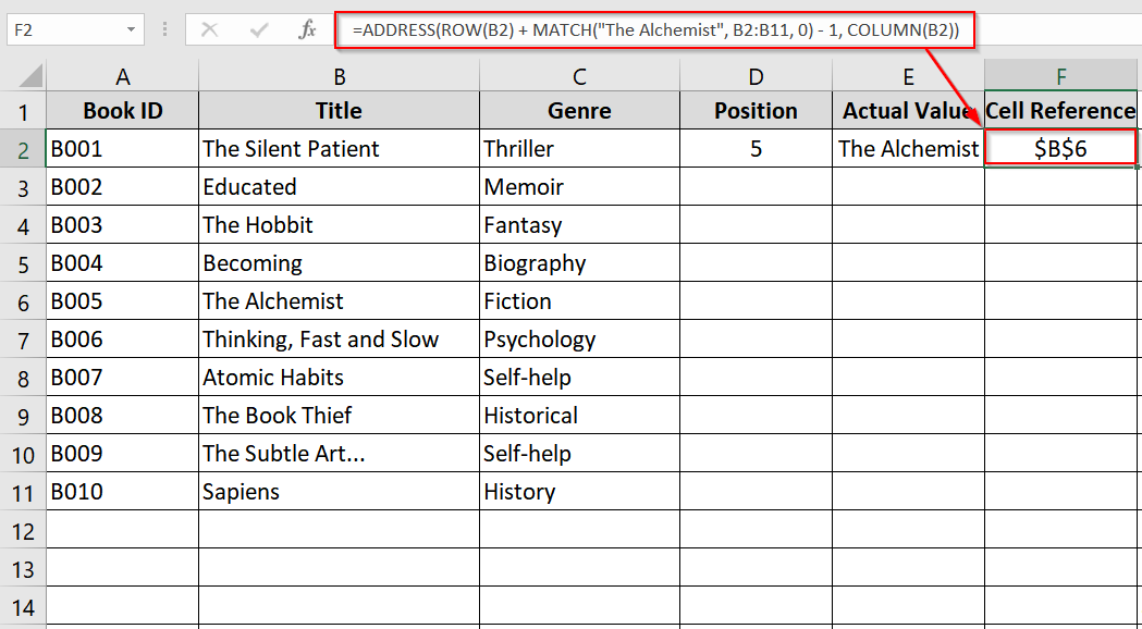
➤ To get the cell reference where the match is found:
=ADDRESS(ROW(B2) + MATCH(“The Alchemist”, B2:B11, 0) – 1, COLUMN(B2))
This returns “B6” because it’s the 5th cell from B2.
Notes:
➧ INDEX(MATCH(…)) gives the value itself.
➧ ADDRESS(ROW + MATCH – 1, COLUMN) returns the cell location.
➧ For horizontal ranges, the logic is the same. You just need adjust the row/column indexing.
Frequently Asked Questions
What is the ISTEXT function in Excel?
ISTEXT(value) checks if a cell contains text. It returns TRUE if the content is text.
How do I find a specific text in a range of cells?
Use SEARCH(“YourText”, range) or MATCH(“YourText”, range, 0) for exact matches.
How do I reference a range of cells in Excel?
You can reference a range using syntax like A2:A10 or dynamically using INDIRECT() or OFFSET().
Concluding Words
I have demonstrated 4 methods on how to find text in range and return cell reference In Excel. Though returning a cell reference instead of a value is an advanced practice but it’s a practical Excel thing. It greatly enhances our data workflows for large and dynamic spreadsheets. You can leave your comment below and I will reply asap.