Duplicate rows are a common issue in Excel. We often encounter repeated entries such as customer names, places, and codes when working on large datasets. This data needs to be removed to avoid inaccurate analysis and overestimation. Whether you are making a report, consolidating vast data, or exporting datasets, you need to remove the duplicate rows based on one column.
To remove duplicate rows from your Excel file, go through the steps below:
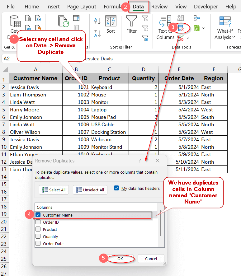
➤ Select any of the cells of your table or a range of cells.
➤ Click on Data tab -> Remove Duplicates.
➤ From the dialog box, mark only the column to which you want to apply the changes.
➤ Click OK to remove the duplicate cells of the specific column.
In this article, we will delve into the basic to advanced methods by which you can remove duplicate rows in Excel. From easy-peasy ways for newbies to automated Power Query methods for professionals, we kept no piece unturned. With our practical tips and chronological guidelines, we’ll have you covered.
Using Excel’s Built-In Remove Duplicates Tool
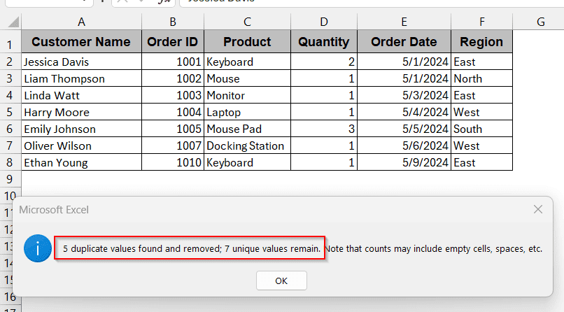
The Excel built-in Remove Duplicate tool is the most efficient option if you are dealing with small databases and don’t require any complexity. It is the best way if you are short on time and looking for one-click cleanup without any advanced features. Here, Excel keeps the first occurrence of the data intact and removes the rest.
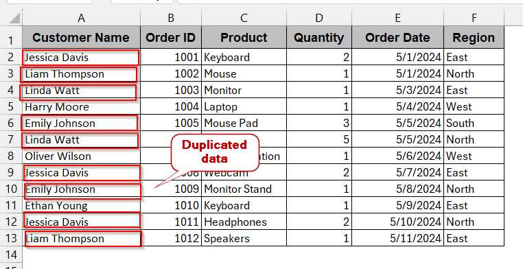
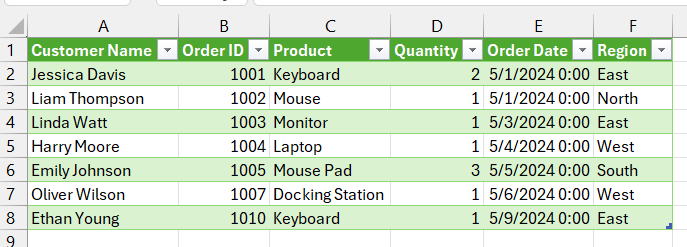
In the below example, we are dealing with the column Customer Name with duplicate data. It has names like Jessica Davis and Linda Watt, which are repeated more than once.
Steps:
➤ In your Excel sheet, select any cell or the entire table.
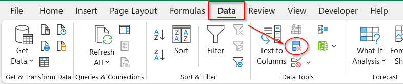
➤ Go to Data -> Remove Duplicate under the Data Tools.
➤ This opens the Remove Duplicate window, showing all the column names.
➤ Choose the column from which you want to remove duplicated data.
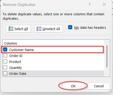
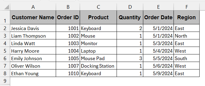
➤ Click OK to proceed. This will remove the duplicate, and your table will look similar to this –
Note:
This method removes the entire row even if only one column has duplicated data.
Delete Duplicate Rows Using Sort and Manual Selection
If you’re working with small datasets and do not want to waste time with formulations and complexity, you can have a look at this method. It is a manual one with a touch of bit of filtering. It works on all versions, does not need prior expertise, and is best for removing duplicates based on one column for minimal data.
Steps:
➤ Select the entire dataset, including all the headers from your Excel file.
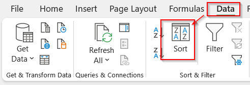
➤ Go to the Data tab and click on the Sort option under Sort and Filter.
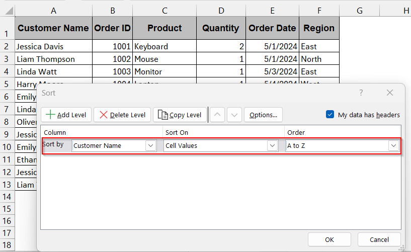
➤ In the Sort dialog box, choose the column name and ensure the sorting order (A to Z, Z to A, or Custom List) depending on your usage.
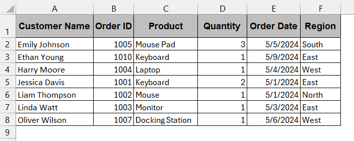
➤ This sorts the table in alphabetical order from A to Z. Seeing this, you can manually remove the row by the Delete option from the right click.
Note:
Always back up your data before starting manual deletion.
Automate Row Deletion Using VBA Macros
As someone having a knack for coding and automation stuff, VBA Macros is the best way for you. With a few lines of code, you can automatically remove duplicate rows with a few simple clicks. This is reusable and works best with the large databases.
Steps:
➤ Go to the Developer tab -> Visual Basic to launch the VBA editor window.
➤ In the window, click on Insert and choose Module from the drop-down menu.
➤ In the blank space, write the code below –
Sub RemoveDuplicatesByColumn()
    Dim ws As Worksheet
    Set ws = ActiveSheet
    Dim lastRow As Long
    lastRow = ws.Cells(ws.Rows.Count, "A").End(xlUp).Row ' Change "A" to your key column
    ws.Range("A1").CurrentRegion.RemoveDuplicates Columns:=1, Header:=xlYes
End Sub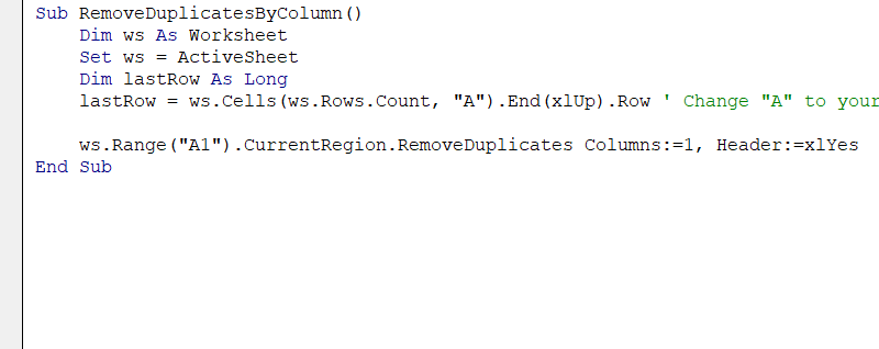
➤ Click Save and close the VBA editor window.
➤ In the Developer tab, choose Macros beside the Visual Basic option.
➤ The Macros window appears; choose the name of the function you just generated (the first line of the code snippet) and click on Run.
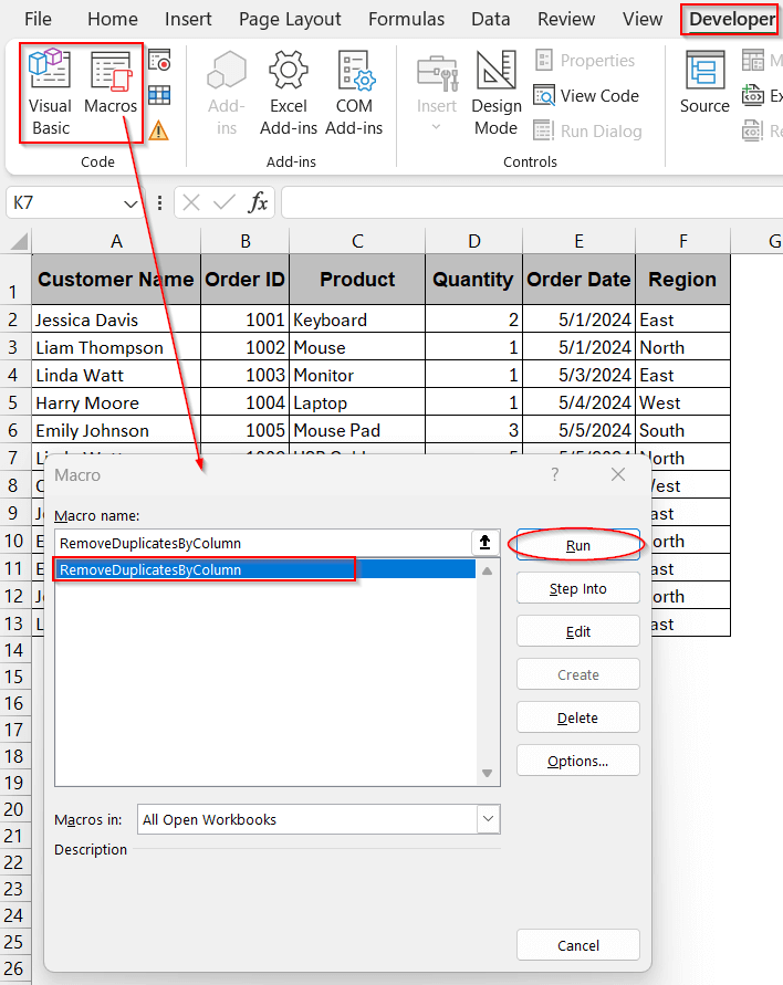
➤ This will automatically remove all the duplicate rows from the table.
Note:
➨ Change A in the code snippet on line 5 with your column –
lastRow = ws.Cells(ws.Rows.Count, “A”).End(xlUp).Row
➨ This code snippet assumes there is a header row in the table.
➨ VBA is an irreversible process. Thus, always have a backup of your data.
Use Power Query to Keep Only Unique Rows in Excel
Manual methods are lengthy and inefficient when you export data repeatedly and regularly. For advanced problems, you need advanced solutions. Power Query tools help you automate and streamline the duplicate values in one column by removing them. It will not only preserve your latest data structure but also smooth the user experience.
Steps:
➤ Select the entire table from the Excel file.
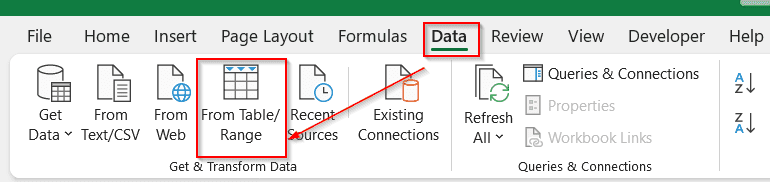
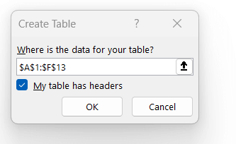
➤ Go to Data -> From Table/Ranges under Get & Transform Data or press Ctrl + T .
➤ The Create Table window appears, confirming the cell range. Mark My table has headers for accurate table creation in Power Query.
➤ This will launch the Power Query window with the table you selected.
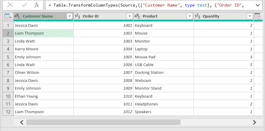
➤ Select the column where you have duplicate data.
➤ Go to the Home Tab and click on Remove Rows under Reduce Rows.
➤ From the dropdown menu, choose the Remove Duplicate option.
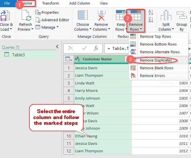
➤ This will remove the entire row where the column Customer Name has any duplicate value.
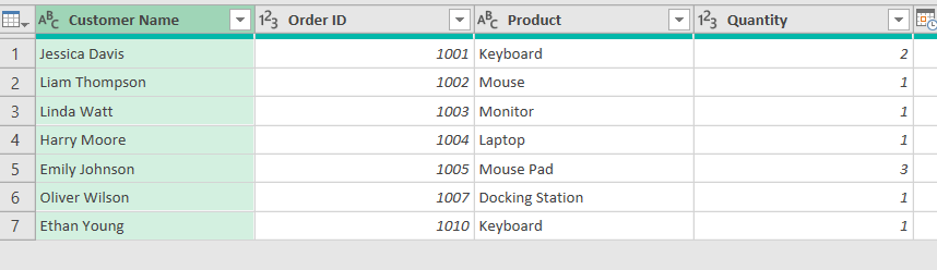
➤ If everything feels right, click on Close & Load located in the left-most part of the Home tab.
➤ This will generate a new worksheet with the new table, with duplicated data removed.
Note:
If you selected multiple columns for duplicate removal, it will be deleted based on the combination of all the columns.
Highlight Duplicate Values Using Conditional Formatting Before Removing
As removing duplicates is an irreversible option, many users become worried about removing them with the built-in tool with just one click. Reviewing them at least once is a better idea. Conditional formatting is the method by which you can first highlight the duplicate values. Without altering any data, you can confirm the data manually in this way.
Steps:
➤ Select the entire column that has duplicate values.
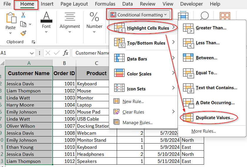
➤ Go to the Home tab and click on Conditional Formatting.
➤ From the dropdown menu, choose Highlight Cell Rule -> Duplicate values.
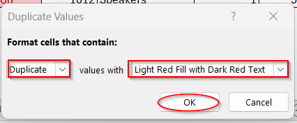
➤ The following window appears to customize the highlight option. Choose as per your requirement.
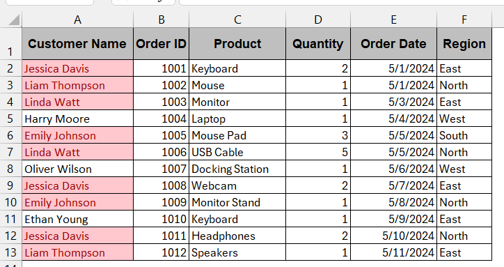
➤ The table will highlight all the duplicate cells in the Customer Name column with a light red fill and red text.
Note:
This method does not remove the data; it highlights all the occurrences of the duplicate values. To remove duplicate cells, use the built-in remove tool or other advanced methods.
Frequently Asked Questions
How do I remove duplicates but keep the last occurrence instead of the first?
The built-in Excel Remove Duplicate option automatically retains the first occurrence and removes the rest of the duplicates. So, to keep the last on instead of first, try to sort the data in descending order at first. Then, you are free to use the native Excel removal tool.
Can I remove duplicates without deleting the whole row?
Excel does not allow you to remove duplicates without deleting the whole row. However, if you want to keep your data intact, you can use functions like UNIQUE or COUNTIF to sort the unique ones separately from each column.
What if duplicates are caused by spaces or formatting differences?
As Excel is case-sensitive, often the same names are not considered duplicates due to space or character differences. To fix that, create a helper row and use the TRIM function to clear space or the UPPER and LOWER functions to make the data case-insensitive.
Is the Remove Duplicates feature case-sensitive?
The Remove Duplicate feature is not case-sensitive. That means it only identifies values when they are identical. For example, ‘Richard’ and ‘richard’ are two different values for this and won’t be recognized as duplicate values.
What’s the difference between Filter Unique and Remove Duplicates?
The main difference between the Filter Unique and the Remove Duplicate is that one removes the duplicates, and the other sorts and filters unique values into a new table.
Can I count how many duplicates I have before removing them?
To count the duplicates in the dataset, you can use the following formula –
=COUNTIF(A:A, A2)
This tells us how many times a value in A2 is repeated in column A. You can know the count of duplicates in this way before removing them.
Concluding Words
Cleaning repeated data is one of the most common data management skills you should have. Using methods like built-in Remove Duplicates to Advanced Filter, and Power Query, it is easy to visualize Excel with removed duplicates. Throughout the article, we tried to explain all the steps and details with key notes, tips, and tricks. If you find anything confusing, download all the workbooks and go through the steps, especially the visuals. Whether you are performing a one-time clean–up or repetitive workflow, you’ll slay it.