Sometimes, Excel cells contain a mix of text and numbers, or a long string of digits where you only want to extract certain numbers. Extracting specific numbers manually can be tedious, but Excel offers several smart ways to get exactly the numbers you need quickly.
In this article, you’ll learn all the best methods to extract specific numbers from a cell in Excel using built-in formulas, Flash Fill, Power Query, and VBA. Whether you want to pull all numbers, just digits in certain positions, or numbers matching a pattern, there’s a working solution for you.
Steps to extract specific numbers from a cell in Excel:
➤ Suppose your mixed data is in cell A2.
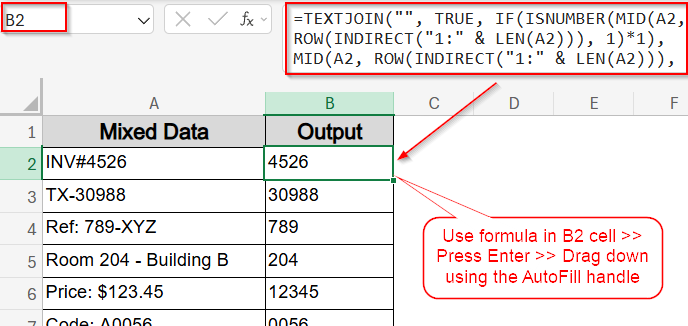
➤ In a blank cell, enter this formula:
=TEXTJOIN(“”, TRUE, IF(ISNUMBER(MID(A2, ROW(INDIRECT(“1:” & LEN(A2))), 1)*1), MID(A2, ROW(INDIRECT(“1:” & LEN(A2))), 1), “”))
➤ For Excel versions earlier than 365, press Ctrl + Shift + Enter to enter it as an array formula. In Excel 365/2021, press Enter.
Use TEXTJOIN Function to Extract Numbers from Any Position
When your data mixes text and numbers like product codes or alphanumeric IDs, it can get difficult to pull just the digits. Excel’s TEXTJOIN function, combined with MID ROW, and INDIRECT offers a smart way to extract all numbers, no matter where they appear.
Steps:
➤ Suppose your mixed data is in cell A2.
➤ In a blank cell, enter this formula:
=TEXTJOIN(“”, TRUE, IF(ISNUMBER(MID(A2, ROW(INDIRECT(“1:” & LEN(A2))), 1)*1), MID(A2, ROW(INDIRECT(“1:” & LEN(A2))), 1), “”))
➤ For Excel versions earlier than 365, press Ctrl + Shift + Enter to enter it as an array formula. In Excel 365/2021, press Enter.
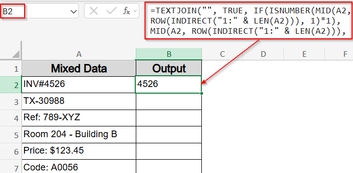
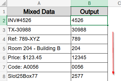
➤ The formula will return only the digits from the original text, concatenated together.
➤ Use the AutoFill handle to drag down the formula to the rest of the cells.
Note:
This formula pulls all digits regardless of position, ignoring letters and special characters.
Extract Numbers from Specific Positions Using MID Function
If the numbers you need are always in the same spot within the string such as characters 3 to 5 in every cell, the MID function is the most efficient approach. It allows you to target a specific start position and pull a fixed number of characters, which is perfect for consistently structured data.
Steps:
➤ Suppose your mixed text data starts in cell A2.
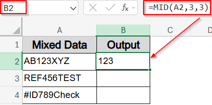
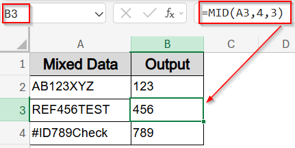
➤ In cell B2, type the following formula to extract the numbers starting from the 3rd character and pulling 3 digits:
=MID(A2,3,3)
➤ Press Enter. This will extract the 3 characters starting from position 3 (i.e., “123” from “AB123XYZ“).
➤ You can adjust the MID formula by changing the starting position and length based on where the number appears. For example, enter this in B3 cell:
=MID(A3,4,3)
This formula pulls 3 digits starting from the 4th character.
➤ Use the AutoFill handle to drag it below to B4 cell since they maintain the same pattern.
Note:
This method works best when the numeric portion is always in the same position across all entries.
Extract Numbers Using Flash Fill (Excel 2013+)
When you don’t want to write formulas and your data follows a visible pattern, Flash Fill can save you time. It recognizes what you’re trying to do based on your first entry and auto-fills the rest.
Steps:
➤ Suppose your mixed data is in column A starting at A2.
➤ In cell B2, manually type the number you want to extract from A2.
➤ Select cell B2 and press Ctrl + E or go to the Data tab >> Flash Fill.
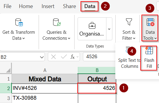
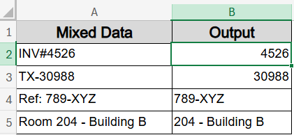
➤ Excel will auto-fill column B with numbers extracted from corresponding cells in column A.
Note:
Flash Fill works well with consistent patterns and is quick without formulas.
Extract Leading Numbers (From Start of Cell)
When numbers appear at the very beginning of a cell and are immediately followed by text, symbols, or spaces, this method helps cleanly pull out just the numeric prefix. It is especially useful for codes, addresses, or any input that starts with digits but contains additional content afterward. There are two formulas you can use, each with distinct behavior.
Using LEFT and SUBSTITUTE
It counts how many numeric characters exist in the entire cell and extracts that many from the left regardless of where they appear. This works only if the digits are guaranteed to be at the very beginning of the string. If other numbers appear later, this method might return extra characters.
Steps:
➤ Assume your mixed data is in the first column starting from A2 cell.
➤ Use this formula in B2 cell:
=LEFT(A2, SUM(LEN(A2) – LEN(SUBSTITUTE(A2, {“0″,”1″,”2″,”3″,”4″,”5″,”6″,”7″,”8″,”9″},””))))
➤ Press Enter and drag down using AutoFill.
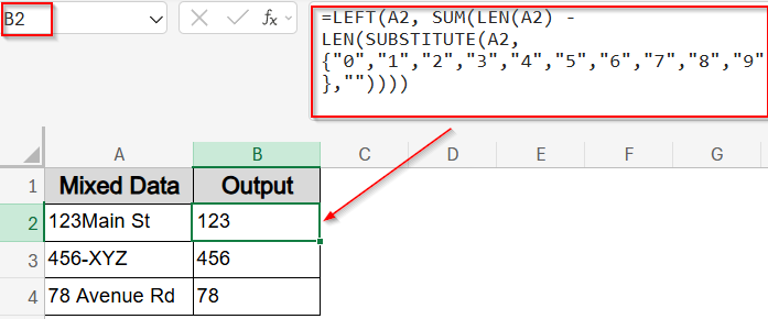
It counts numeric characters and grabs that many from the left.
Combining LEFT with MATCH and MID
This formula scans the text one character at a time from the start and stops at the first non-numeric character. It ensures only the leading digits are captured and is more reliable when the string contains additional numbers later. Use this when your data may include embedded or trailing numbers and you only want the initial block.
Steps:
➤ Use formula in a blank cell like B2:
=LEFT(A2, MATCH(FALSE, ISNUMBER(MID(A2, ROW(INDIRECT(“1:”&LEN(A2)+1)), 1) *1), 0) -1)
➤ Press Enter and drag down using AutoFill.
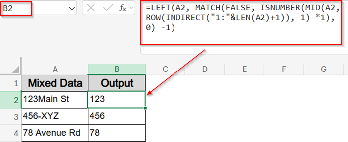
Now the first non-digit is found and digits before it are extracted.
Extract Number in the Middle or Between Characters
When numbers appear between characters like colons, dashes, or brackets, you can use functions like MID, TEXTAFTER, TEXTBEFORE and others to extract only the enclosed numeric values cleanly. Let’s get started.
Extract Numbers Inside Parentheses
Use this when numbers are inside parentheses, such as (456). This method pinpoints bracket positions and extracts just the content between them accurately.
Steps:
➤ Use this formula in a blank cell like B2 if your data begins from A2:
=MID(A2, FIND(“(“, A2)+1, FIND(“)”, A2)-FIND(“(“, A2)-1)
➤ You can adjust the formula for other bracket types by placing it inside the double quotation (” “) sign.
➤ Press Enter and drag down using AutoFill.
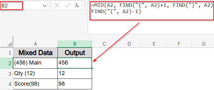
Now this locates both parentheses and pulls out the digits in between using relative character positions.
Extract Numbers After Specific Characters
This method is great when your data uses consistent labels like “Qty:“, “Score:“, or “Price:“. It extracts the number that appears right after a known text string and stops at the next space or delimiter.
Steps:
➤ Use this formula in a blank cell like B2 if your data begins from A2:
=TEXTBEFORE(TEXTAFTER(A2, “Qty: “), ” “)
➤ Press Enter and drag down using AutoFill.
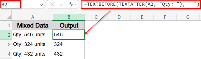
This extracts digits after “Qty:” and before the next space.
Extract Numbers After a Specific Delimiter
When a consistent delimiter like a colon separates labels from numbers (e.g., “Score: 8”), this method captures everything that appears after that specific character.
Steps:
➤ Use this formula in a blank cell like B2 if your data begins from A2:
=TRIM(MID(A2, FIND(“:”, A2)+1, LEN(A2)))
➤ Press Enter and drag down using AutoFill.
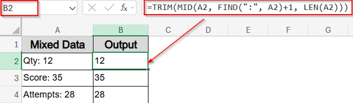
This finds the colon and extracts everything after it, removing extra spaces using TRIM function.
Extract Trailing Numbers (From End of Cell)
When numbers appear consistently at the end of your cell content, such as product IDs or customer codes, this method helps isolate just that trailing numeric portion. It’s best used when the end of your string is always the number, and the preceding content may vary in length or characters. Let’s look at some working formulas.
Using RIGHT and SEARCH
This formula finds the position of the first digit and pulls all characters from that point to the end which is useful if digits always trail, regardless of character type before them.
Steps:
➤ Use this formula in a blank cell like B2 if your data begins from A2:
=RIGHT(A2, LEN(A2) – MIN(SEARCH({0,1,2,3,4,5,6,7,8,9}, A2 & “0123456789”)) + 1)
➤ Press Enter and drag down using AutoFill.
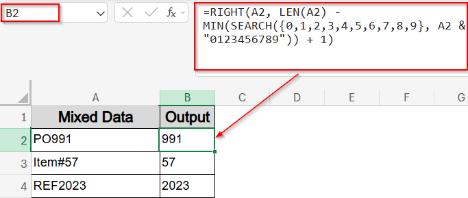
Now this detects the first number and pulls till the end.
Combining RIGHT with ISNUMBER
This version locates the last non-digit character and extracts everything after it, ensuring only the trailing numeric part is returned. More accurate when letters or symbols precede the number.
Steps:
➤ Use this formula in a blank cell like B2 if your data begins from A2:
=RIGHT(A2, LEN(A2) – MAX(IF(ISNUMBER(MID(A2, ROW(INDIRECT(“1:”&LEN(A2))), 1) *1)=FALSE, ROW(INDIRECT(“1:”&LEN(A2))), 0)))
➤ Press Enter and drag down using AutoFill.
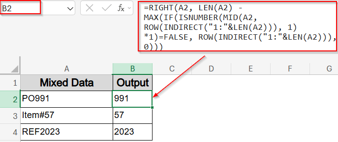
Now this locates the last non-digit and extracts the numeric tail.
Extract First Number Group (For Dynamic Position)
If your cell contains alphanumeric content with numbers appearing in unpredictable places like RefABC123XYZ456 or UserID007Name, this method helps extract the first full block of digits, no matter where it starts. It dynamically detects the first numeric sequence and pulls only that portion, ignoring any text or symbols before or after.
Steps:
➤ Use this formula in a blank cell like B2 if your data begins from A2:
=LET(
txt, A2,
pos, MATCH(TRUE, ISNUMBER(–MID(txt, SEQUENCE(LEN(txt)), 1)), 0),
len, MATCH(FALSE, ISNUMBER(–MID(txt, SEQUENCE(LEN(txt)-pos+1)+pos-1, 1)), 0) – 1,
VALUE(MID(txt, pos, len))
)
➤ Press Enter and drag down using AutoFill.
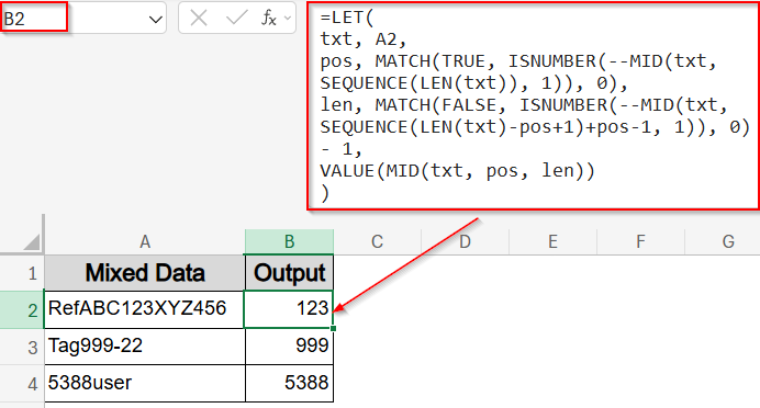
This finds the first digit block and extracts it as a number.
Extract Numbers from Product Codes (For Dash or Prefix)
When product codes use symbols like dashes or underscores before the numeric part (e.g., ITEM-5678), this method locates the separator and extracts the digits that follow, regardless of text length or format.
Steps:
➤ Use this formula in a blank cell like B2 if your data begins from A2:
=RIGHT(A2, LEN(A2) – FIND(“-“, SUBSTITUTE(A2, MID(A2, MIN(FIND({“0″,”1″,”2″,”3″,”4″,”5″,”6″,”7″,”8″,”9″}, A2&”0123456789”)), 1), 1)))
➤ Press Enter and drag down using AutoFill.
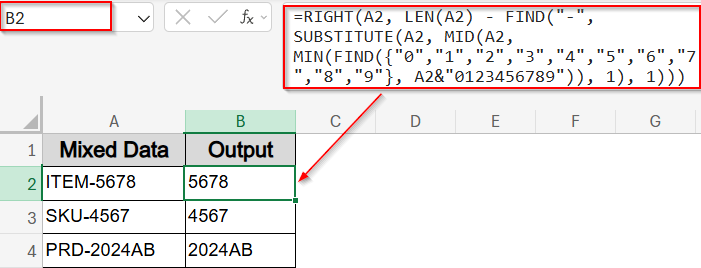
This formula dynamically finds digits after dash and extracts them.
Extract Numbers Including Decimals
When numbers in your data include decimal points such as currency values, use this method to keep the entire number.
Steps:
➤ Use this formula in a blank cell like B2 if your data begins from A2:
=TEXTJOIN(“”, TRUE, IFERROR(
IF(MID(A2, ROW(INDIRECT(“1:” & LEN(A2))), 1)=”.”, “.”,
IF(ISNUMBER(–MID(A2, ROW(INDIRECT(“1:” & LEN(A2))), 1)),
MID(A2, ROW(INDIRECT(“1:” & LEN(A2))), 1),
“”)
),””))
➤ Press Enter and drag down using AutoFill.
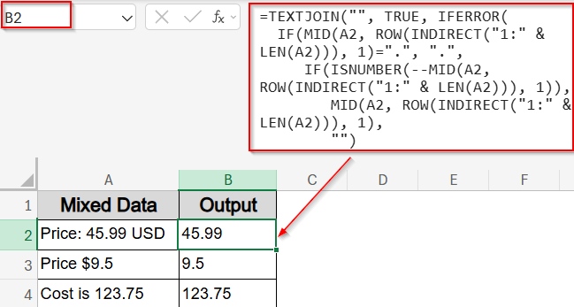
This extracts numeric characters and a single decimal dot.
Extract Using REGEX (For Excel 365+)
Using the REGEX function is the cleanest way to pull structured number formats, including commas or decimals. Ideal for financial or numeric reports.
Steps:
➤ Use this formula in a blank cell like B2 if your data begins from A2:
=REGEXEXTRACT(A2, “\d[\d,\.]*”)
➤ Press Enter and drag down using AutoFill.
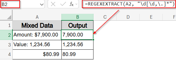
This captures formatted numbers including comma/decimal.
Extract Using SUMPRODUCT (For Scattered Digits)
When digits are scattered throughout a text string in no specific order like in A2B3C4 or 9X8Y7, this advanced array formula uses SUMPRODUCT function to locate numeric characters, assign their positions, and reconstruct the full number. It’s especially useful in older Excel versions where functions like TEXTJOIN or LET aren’t available.
Steps:
➤ Use this formula in a blank cell like B2 if your data begins from A2:
=SUMPRODUCT(MID(0&A2,LARGE(INDEX(ISNUMBER(–MID(A2,ROW($1:$20),1))*ROW($1:$20),0),ROW($1:$20))+1,1)*10^(ROW($1:$20)-1))
➤ Press Enter and drag down using AutoFill.
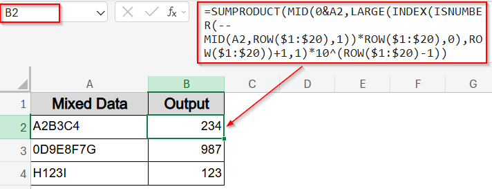
This reconstructs a number by calculating the digit positions.
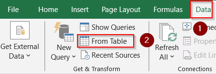
Extract Numbers Using Power Query for Complex Patterns
Power Query is excellent for extracting numbers when your data has complex patterns or multiple numbers per cell.
Steps:
➤ Select your data range and go to the Data tab >> Get & Transform group >> From Table/Range.
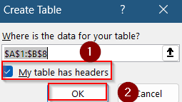
➤ In the dialog, check your headers and click OK.
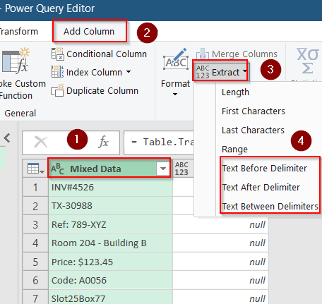
➤ In Power Query Editor, select the column with mixed text.
➤ Go to Add Column >> Extract >> Text Between Delimiters or use Extract > Text Before/After Delimiter depending on the pattern.
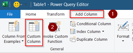
➤ For advanced extraction, go to Add Column >> Click Custom Column.
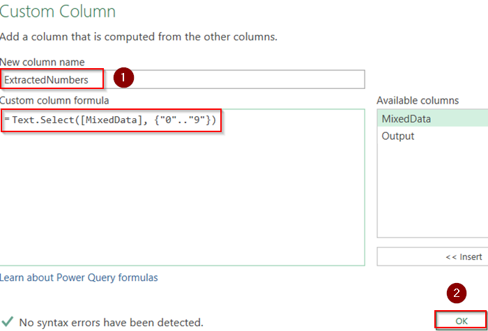
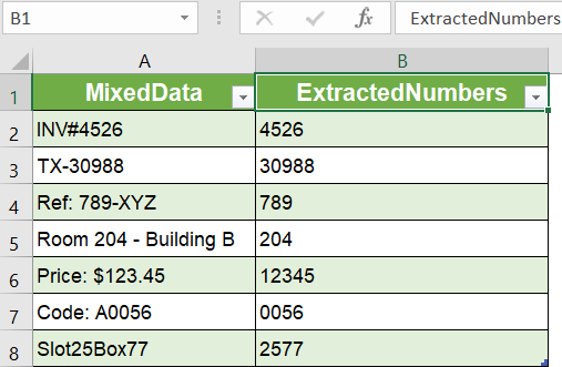
➤ Name the column ExtractedNumbers and add a Custom column formula like this:
=Text.Select([MixedData], {“0”..”9″})
Here, replace MixedData with your column name.
➤ Click OK to confirm.
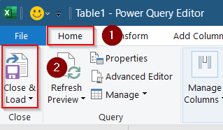
➤ Click Close & Load under Home tab to return the cleaned data to Excel.
Now your extracted numbers are loaded into a new sheet as a Table.
Use VBA to Extract Numbers From a Cell Automatically
For frequent or bulk extraction, VBA lets you create a macro that pulls out numbers from text cells.
Steps:
➤ Press Alt + F11 to open the VBA editor.
➤ Insert a new Module via Insert >> Module.
➤ Paste the following code:
Function ExtractNumbers(cell As Range) As String
    Dim chars As String, i As Integer, result As String
    chars = cell.Value
    For i = 1 To Len(chars)
        If Mid(chars, i, 1) Like "[0-9]" Then
            result = result & Mid(chars, i, 1)
        End If
    Next i
    ExtractNumbers = result
End Function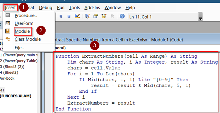
➤ Close the editor and use the formula in Excel like:
=ExtractNumbers(A2)
➤ Drag down using the AutoFill handle.
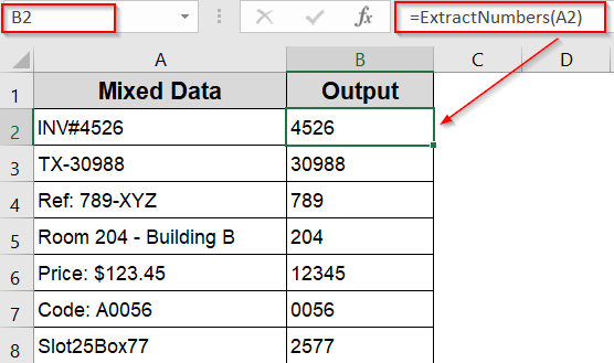
This UDF (User Defined Function) returns all numbers concatenated from the cell.
Frequently Asked Questions
How do I extract only numbers from mixed text like “ABC123XYZ”?
You can use Excel formulas that scan each character in a cell, identify digits, and join them together, effectively removing all letters and special characters to leave just the numbers like the TEXTJOIN function.
Can I extract numbers that appear between parentheses or other symbols automatically?
Yes, by using functions like MID and FIND to locate the positions of specific characters like parentheses. Then Excel can extract the exact content inside, including numbers between those symbols without manual effort.
What’s the best way to extract numbers when digits appear randomly anywhere in a string?
Dynamic formulas using LET function can detect the first continuous block of digits in any position within the text, extracting just that number group without needing the digits to be in fixed places.
Wrapping up
In this tutorial, we learned how to extract specific numbers from a cell in Excel using a variety of methods starting from simple formulas like MID and LEFT to advanced functions and tools like LET, REGEX, VBA and Power Query. We also covered practical cases like extracting numbers after labels, from between characters, or only from consistent positions. Feel free to download the practice file and share your feedback.