If you’re dealing with a dataset that’s spread horizontally across rows but needs to be reorganized into vertical columns, you’re not alone. Excel doesn’t always give you data in the perfect shape, especially when you’re importing reports or combining inputs from various sources. Fortunately, Excel offers multiple ways to reshape your data with ease.
In this article, you’ll learn all the best methods to convert multiple rows to columns in Excel using Paste Special, formulas, Power Query, and even VBA for automation.
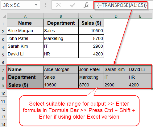
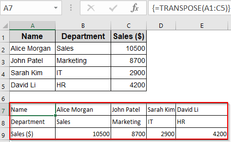
➤ Select the suitable data range where you want your output.
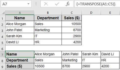
➤ Go to the formula bar at top and type the formula: =TRANSPOSE(A1:C5)
➤ In earlier Excel versions, press Ctrl + Shift + Enter to enter it as an array formula and for newer Excel versions press only Enter.
➤ Your transposed data will be visible instantly. You can additionally format it according to your preferences.
Transpose Rows to Columns Instantly Using Paste Special
This method is best for users who want a quick and manual way to convert rows into columns. It’s ideal when you don’t need your data to stay linked to the original.
Steps:
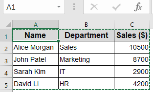
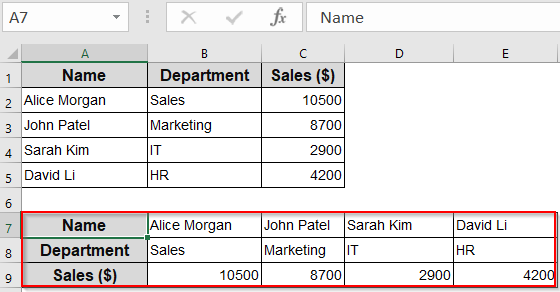
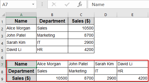
➤ Select the rows you want to convert. For example, highlight cells A1:C5.
➤ Press Ctrl + C to copy the selection.
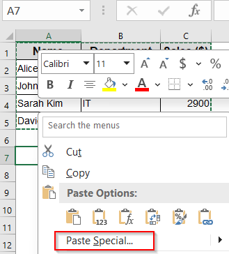
➤ Right-click on a blank area of your sheet (e.g., A7) and choose Paste Special.
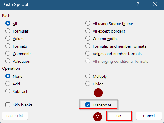
➤ In the Paste Special dialog, check the Transpose box at the bottom.
➤ Click OK.
Your selected rows will now appear as columns. Note that the pasted data is static, so changes in the original range won’t reflect in the transposed version.
Note:
Your data will be transposed without any formatting. You need to manually format it afterwards.
Use TRANSPOSE Function (Dynamic Link)
This method is great when you want the transposed data to stay linked to the original. Any changes made to the source rows will automatically update in the converted columns.
Steps:
➤ Select a blank area in your worksheet where you want to output the data. Make sure it’s sized appropriately to fit the transposed version such as A7:E9.
➤ Type the following formula in the Formula Bar at top:
=TRANSPOSE(A1:C5)

➤ In Excel 365 or Excel 2021, press Enter. In earlier versions, press Ctrl + Shift + Enter to enter it as an array formula.
➤ Excel will now display your rows as columns, keeping them dynamically linked to the original data.
➤ You can now format your data accordingly.
Use this when maintaining live connections between row-based and column-based formats is important.
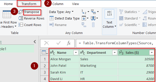
Convert Rows to Columns Using Power Query
If you’re working with large datasets or doing frequent row-to-column transformations, Power Query gives you more control. It’s especially useful for pivot-style reformatting.
Steps:
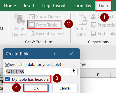
➤ Select your data and go to the Data tab on the ribbon.
➤ Click From Table/Range. If prompted, confirm your data range and check the “My table has headers” option.
➤ Once inside Power Query, select the columns you want to pivot.
➤ Go to the Transform tab, and click Transpose.
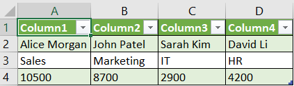
➤ Click Close & Load to bring the transformed data back into your worksheet.
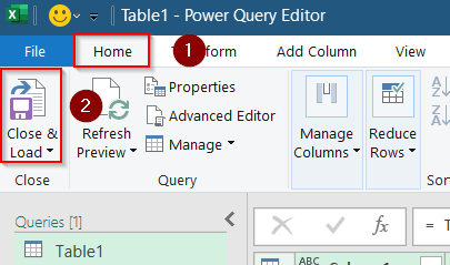
Now you have a new table with your rows converted into columns. You can refresh it anytime your source data changes.
Use VBA to Convert Rows to Columns Automatically
If you regularly convert rows to columns across multiple sheets or workbooks, a VBA macro can automate the task and save you tons of time.
Steps:
➤ Press Alt + F11 to open the VBA editor.
➤ In the left pane, right-click on VBAProject (YourWorkbookName) and insert a new Module.
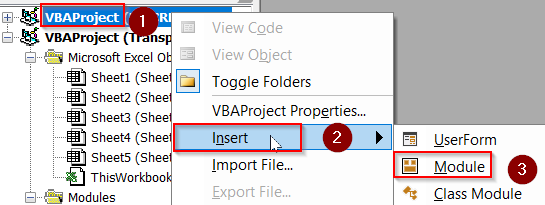
➤ Paste the following code in the blank box that appears:
Sub ConvertRowsToColumns()
    Dim rng As Range
    Dim outCell As Range
    Set rng = Range("A1:C5") ' Set your row range
    Set outCell = Range("A7") ' Output start cell
    rng.Copy
    outCell.PasteSpecial Paste:=xlPasteAll, Transpose:=True
End Sub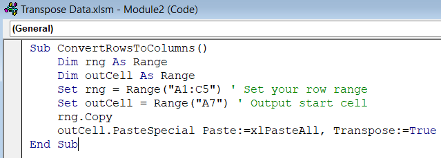
➤ Update the range references (A1:C5, A7) as needed.
➤ Press F5 key to run the macro manually. Your rows will be transposed into columns instantly.
➤ Additionally, you can manually adjust the formatting according to your liking.

This method is perfect for automating repetitive tasks or building custom Excel tools.
Frequently Asked Questions
Can I convert rows to columns and still keep the formatting?
Yes, but the Paste Special method doesn’t always copy formatting. Use Power Query or apply formatting manually after pasting.
Is there a limit to how many rows I can transpose?
Technically yes, Excel has a row/column limit. If your data exceeds available columns after transposing, you may hit the limit.
Does the TRANSPOSE function work with merged cells?
No, the TRANSPOSE function does not support merged cells. Unmerge them before applying the function.
Can I use formulas to convert rows to columns beyond TRANSPOSE?
Not directly, but advanced users sometimes use INDEX or OFFSET for customized reshaping, though TRANSPOSE is still the easiest.
Wrapping Up
In this tutorial, you learned how to convert multiple rows to columns in Excel using various approaches: from the simple Paste Special option to dynamic formulas, Power Query, and automation via VBA. Feel free to download the practice file and share your feedback.