
Users using Google Sheets often want to move data from one sheet to another. This is when the IMPORTRANGE function comes in handy. But sometimes, the user only wants to import certain rows that meet certain criteria, like a certain category, status, or date. In those situations, you need to use the IMPORTRANGE function with specific conditions. It’s especially helpful for making dashboards, departmental reports, shared sheets where roles limit data visibility, or just getting rid of extra data that isn’t needed.
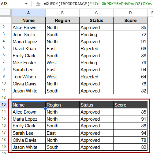
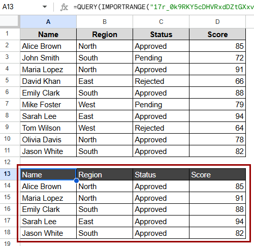
➤ In the destination sheet (Sheet6), click on a blank cell. In this case, A13.
➤ Use the formula:
=QUERY(IMPORTRANGE(“17r_0k9RKY5cDHVRxdDZtGXxvuTIjg15X10eodipx3So”, “Sheet1!A1:D”), “SELECT Col1, Col2, Col3, Col4 WHERE Col3 = ‘Approved'”, 1)
➤ Press Enter to apply the function and see the filtered imported data.
We will look at several ways to use IMPORTRANGE with conditions in Google Sheets in this article. These include basic QUERY integration, using multiple conditions, applying helper columns, and combining with FILTER. We’ll also answer some of the most common questions that people have about how to fix or improve their use.
Overview of the IMPORTRANGE Function in Google Sheets
IMPORTRANGE function in Google Sheets lets you bring in a range of data from another spreadsheet. The basic syntax is
=IMPORTRANGE(“spreadsheet_url”, “range_string”)
Here, “spreadsheet_url” is the full URL of the source sheet, and “range_string” tells you the name of the sheet and the range (for example, “Sheet1!A1:D100“).
But IMPORTRANGE pulls in all the data without any filtering or conditions. That’s when it becomes powerful to combine it with QUERY.
Using QUERY Function with IMPORTRANGE for Conditional Import
This method applies the QUERY function and IMPORTRANGE to only bring in certain rows that meet a certain condition. It operates best when you want to filter imported data based on the value of just one column. This method lets you control which data gets efficiently pulled into your current spreadsheet by using SQL-style syntax.
This example shows a shared spreadsheet with records of sales in Sheet1. We only want to bring in rows where the “Status” says “Approved.”

Steps:
➤ In the destination sheet (Sheet2), click on A13, a blank cell.
➤ Use the formula:
=QUERY(IMPORTRANGE(“17r_0k9RKY5cDHVRxdDZtGXxvuTIjg15X10eodipx3So”, “Sheet1!A1:D”), “SELECT Col1, Col2, Col3, Col4 WHERE Col3 = ‘Approved'”, 1)
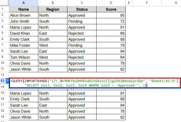
➤ Press Enter.
➤ If you are asked, click Allow Access after pasting the formula. This will only give you data where the “Status” column says “Approved.”

Note:
You have to put text values in single quotes (‘Approved’) inside the QUERY at all times.
Applying Multiple Conditions with IMPORTRANGE
This method is excellent when you need to import data based on more than one condition, like when you want to utilize a text filter and a numerical threshold together. It builds on combining the QUERY and IMPORTRANGE methods but adds logical operators like AND and OR to complicate filters.
This method lets you import data from another spreadsheet as long as more than one condition is met, such as the Status being “Approved” and the Score being higher than 80.
Steps:
➤ In the destination sheet (Sheet3), click on a blank cell. Here, A13.
➤ Enter the formula:
=QUERY(IMPORTRANGE(“17r_0k9RKY5cDHVRxdDZtGXxvuTIjg15X10eodipx3So”, “Sheet1!A1:D”), “SELECT Col1, Col2, Col3, Col4 WHERE Col3 = ‘Approved’ AND Col4 > 80”, 1)

➤ Press Enter. The results will exclude data with a “Score” under 80 and any data that has not been “Approved” in the “Status” column.

Note:
You can use AND/OR within the QUERY function, similar to SQL. While applying more than one comparison, your column index should align with the imported range’s arrangement.
Using Helper Columns for More Complex Conditions
There are times when the logic you want to use is too complicated or cluttered to fit into one QUERY formula. In these situations, helper columns in the source sheet can make things easier. This method adds a new column that marks or labels rows to be imported based on conditions that you set. Next, IMPORTRANGE and QUERY bring in only the marked rows, ensuring the destination sheet remains clean and easy to work with.
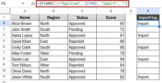
If you want to import only the entries that are both “Approved” as well as scored above 80, but you don’t want to use complicated formulas in your destination file.
Steps:
➤ In your source sheet, create a new column (e.g., Column F) titled ImportFlag.
➤ Type this formula in cell F2 and drag it down:
=IF(AND(C2=”Approved”, D2>80), “Import”, “”)
➤ Now go to your destination sheet (Sheet4) and use this formula:
=QUERY(IMPORTRANGE(“17r_0k9RKY5cDHVRxdDZtGXxvuTIjg15X10eodipx3So”, “Sheet1!A1:F”), “SELECT Col1, Col2, Col3, Col4 WHERE Col6 = ‘Import'”, 1)

➤ Press Enter.
Note:
By calculating them in the source sheet, this method makes complicated conditions easier to understand. You can use more advanced logic in the helper column without making the QUERY function too complicated.
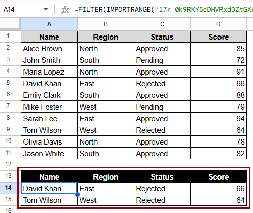
Combining FILTER with IMPORTRANGE
You can use FILTER with IMPORTRANGE instead of QUERY to make conditions that are easier to understand and work with, especially if you want case-insensitive filtering or want to keep the original headers. It can take more work to repeat the IMPORTRANGE function for the condition column, but it lets you evaluate rows more flexibly without the SQL-like syntax of QUERY.
We can easily get only the rows where the status is “Rejected” by using FILTER with IMPORTRANGE.
Steps:
➤ In the destination sheet (Sheet5), click on a blank cell.
➤ Apply this formula:
=FILTER(IMPORTRANGE(“17r_0k9RKY5cDHVRxdDZtGXxvuTIjg15X10eodipx3So”, “Sheet1!A1:D”), IMPORTRANGE(“17r_0k9RKY5cDHVRxdDZtGXxvuTIjg15X10eodipx3So”, “Sheet1!C1:C”) = “Rejected”)
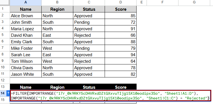
➤ Press Enter. The result will show the entries where the status is “Rejected.”
Note:
For the filtered column, you need to call IMPORTRANGE separately. The number of rows must be the same. There won’t be any headers, so you might have to add them by hand to the destination sheet.
Frequently Asked Questions
What does “Unable to parse query string” mean when using IMPORTRANGE?
This mistake usually means that your QUERY syntax is wrong. Make sure you utilize the right quotes around text conditions and double-check the names of the columns (Col1, Col2, etc.).
How do I use a date condition with IMPORTRANGE?
Your query should look like this if you want to filter by date:
“SELECT Col1 WHERE Col4 > date ‘2024-01-01′”
Check that the date column is set up correctly in the source sheet.
Can I reference a cell for the condition instead of typing it?
QUERY doesn’t let you directly reference cells from other sheets. You can, however, build the query dynamically by using concatenation like this:
=QUERY(IMPORTRANGE(“url”, “range”), “SELECT Col2 WHERE Col3 = ‘” & A1 & “‘”, 1)
Does IMPORTRANGE update automatically when source data changes?
Yes, IMPORTRANGE is a dynamic function that updates on its own. But depending on how big and complicated your sheet is, there may be a small delay.
Can I import only visible rows after a filter with IMPORTRANGE?
No, IMPORTRANGE imports the whole range, no matter what filters are set in the source. To simulate filtering, you would have to use QUERY.
Is there a limit to how many cells IMPORTRANGE can fetch?
Yes, Google Sheets has a limit of 50,000 to 100,000 cells per spreadsheet and certain limits on how many functions can be run at once. Don’t import datasets that are too big for no reason.
Concluding Words
IMPORTRANGE makes it easy to manage and show filtered data across spreadsheets. This method allows you to control what gets pulled in in a flexible way when importing, based on one or multiple conditions. Using helper columns makes the logic easier to understand while making the text easier to read when the needs are more complicated.