Need to track upcoming deadlines, events, or tasks in your spreadsheet? Google Sheets lets you use conditional formatting to highlight dates that fall within the next 7 days automatically. This is especially useful for project timelines, to-do lists, or event schedules.
In this article, we’ll show you multiple ways to apply conditional formatting rules that highlight dates falling within the next 7 days, using functions like TODAY, ISDATE, AND, and logical operators.
Steps to highlight dates within the next 7 days in Google Sheets using the TODAY and AND functions in conditional formatting:
➤ Use the dataset in a cell range, such as C2:C8, where the Due Dates are listed.
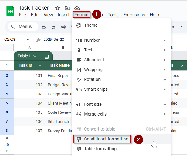
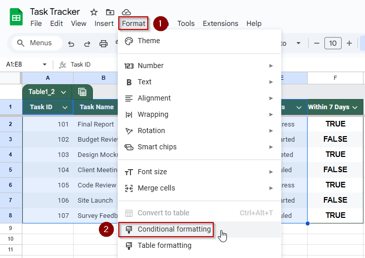
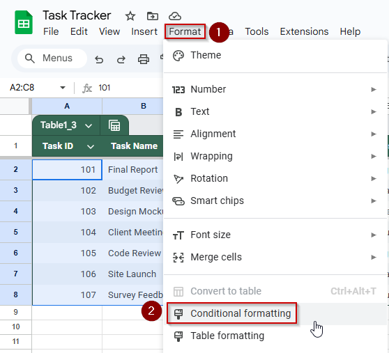
➤ Select the range C2:C8 and go to Format >> Conditional formatting.
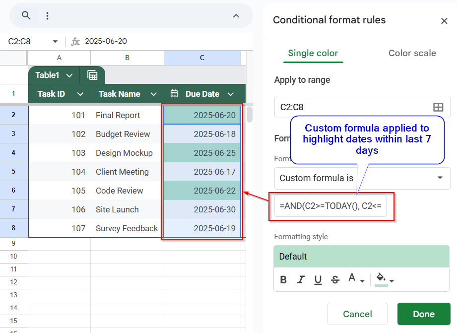
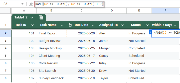
➤ Under Format rules, choose Custom formula is, and enter this formula:
=AND(C2 >= TODAY(), C2 <= TODAY() + 7)
➤ Choose a formatting style to highlight cells that meet the criteria.
➤ Click Done to apply the rule and highlight upcoming dates automatically.
Highlight Dates Within the Next 7 Days
This method uses a custom formula in Google Sheets’ conditional formatting to automatically highlight dates that fall within the next 7 days from today. By combining the TODAY function with the AND function, it checks whether each date is not in the past and occurs within a week ahead. This dynamic approach helps you quickly spot upcoming deadlines or events without manual date tracking.
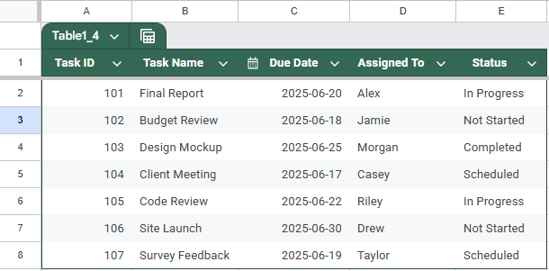
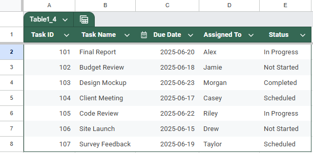
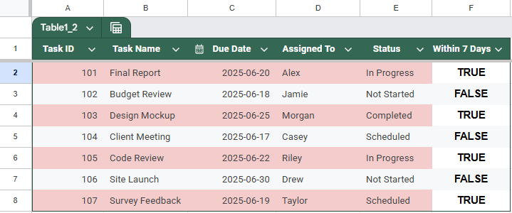
This is the dataset we will be using for the article:
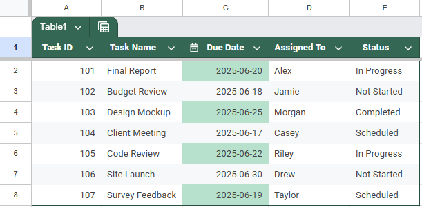
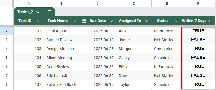
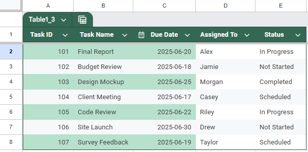
The output will highlight all cells in your selected date range that contain a date between today and the next 7 days, making upcoming deadlines or events stand out visually.
Steps:
➤ Select the range of Due Dates in your sheet: C2:C8.
➤ Go to Format >> Conditional formatting.

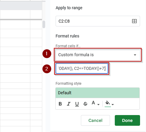
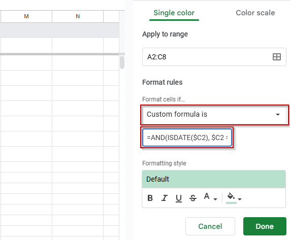
➤ Under Format rules, choose Custom formula is.
➤ Enter this formula:
=AND(C2>=TODAY(), C2<=TODAY()+7)
➤ Choose a formatting style (like a background color or text color) to highlight matching cells.
➤ Click Done.
➧ C2<=TODAY()+7 checks if the date is within 7 days from today.
➧ The AND() function combines these conditions so only dates that satisfy both get highlighted.
➧ Applying this rule to the Due Date column will highlight all tasks due within the next week.
Automatically Highlight Recent Dates from the Past 7 Days
This method uses a custom formula with the AND, TODAY, and ISDATE functions in Google Sheets’ conditional formatting to highlight cells containing dates that fall within the past 7 days (excluding today). It gives you precise control, unlike preset options, and is perfect for tracking recent activity such as submissions, updates, or events that occurred within the last week.
This is the updated dataset that we will be using for this method:
Steps:
➤ Select the range C2:C8 in your sheet.
➤ Go to Format >> Conditional formatting.
➤ Under Format cells if, choose Custom formula is.
➤ Enter this formula:
=AND(C2<TODAY(), C2>=TODAY()-7, ISDATE(C2))
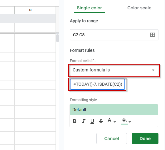
➧ C2>=TODAY()-7 ensures the date is no more than 7 days old.
➧ ISDATE(C2) confirms the cell contains a valid date.
➤ Pick a formatting style (like a red fill or bold text) to make the highlighted cells stand out.
➤ Click Done.
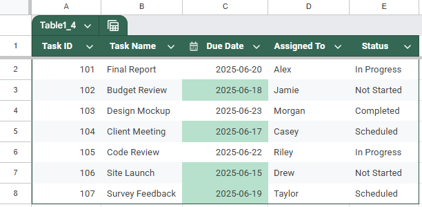
This method will highlight cells with dates that fall within the past 7 days.
Apply Conditional Formatting Using a Helper Column in Google Sheets
If you want more control or need to apply multiple complex conditions, using a helper column is a clean and flexible approach. In this method, you’ll calculate whether each date falls within the next 7 days in a separate column, and then apply conditional formatting based on that column’s value. This keeps formulas simple inside the formatting rule and makes debugging easier.
Steps:
➤ Suppose your dates are in column C (C2:C8). In column F, label cell E1 as “Within 7 Days”.➤ In cell F2, enter the following formula:
=AND(C2 >= TODAY(), C2 <= TODAY() + 7)
➤ Drag the formula down to fill for all rows with data. TRUE indicates the date is within the next 7 days.
➤ Now, select the range A2:E8 (or your full data range).
➤ Go to Format >> Conditional formatting.
➤ Under “Format rules”, choose Custom formula is and enter:
=$F2=TRUE
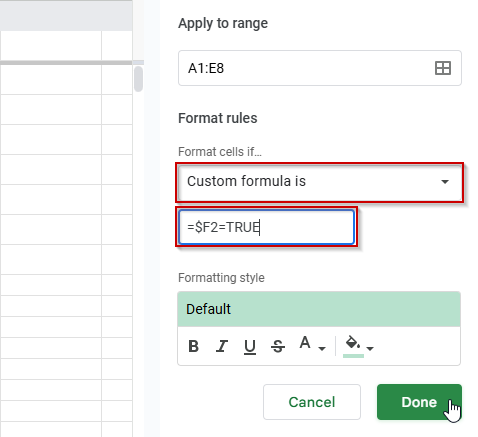
➤ Set your desired formatting style and click Done.
➧ Conditional formatting reads this column to decide which rows to highlight.
➤ This method is especially useful when combining multiple conditions or debugging formula logic.
Combine ISDATE and AND Functions in Conditional Formatting
When working with mixed data or user-input cells, it’s common to encounter invalid or blank entries. Using the ISDATE function along with AND helps ensure that conditional formatting only applies to valid date values that fall within your desired range, like the next 7 days. This approach avoids errors and misformatting, especially in collaborative or form-fed sheets.
Steps:
➤ Assume your dates are in column C, from cells C2 to C8.
➤ Select the range A2:C8 (or your complete data rows).
➤ Go to Format >> Conditional formatting.
➤ Under “Format rules,” choose Custom formula is and enter:
=AND(ISDATE($C2), $C2 >= TODAY(), $C2 <= TODAY() + 7)
➤ Choose your preferred formatting style (e.g., background color) and click Done.
➧ C2 >= TODAY() and C2 <= TODAY() + 7 ensure the date falls within the next 7 days.
➤This method prevents conditional formatting from applying to invalid entries or blank rows, improving accuracy in real-world datasets.
Frequently Asked Questions
What does the TODAY() function do in Google Sheets?
The TODAY() function returns the current date and updates automatically each day, making it ideal for dynamic conditional formatting or time-based formulas.
Why isn’t my conditional formatting working with dates?
Your column might be formatted as text. Ensure cells are properly set to “Date” format. Also, check that your formula references the top-left cell in the selected range.
Can I highlight weekends separately from weekdays within the next 7 days?
Yes. Use =WEEKDAY(C2, 2) > 5 in conditional formatting to highlight weekends (Saturday and Sunday), even within a 7-day date range.
Will this method update automatically each day?
Yes. Since the formula uses TODAY, it recalculates daily. Dates that newly fall within the 7-day range will automatically be highlighted, and expired ones will be cleared.
Wrapping Up
Highlighting dates within the next 7 days using conditional formatting in Google Sheets is a powerful way to track upcoming tasks, deadlines, or events with dynamic formulas, such as TODAY and AND, ensuring your spreadsheet always reflects real-time urgency with no manual updates required. Whether you’re managing projects or reminders, this method keeps your timeline visually clear and actionable.