Google Sheets has several powerful tools, but Conditional Formatting is something extraordinary.
With the Conditional Formatting, you can easily highlight cells of your choice and smartly present the spreadsheet. This article will show multiple conditional formatting applications that will smooth your spreadsheet presentation journey.
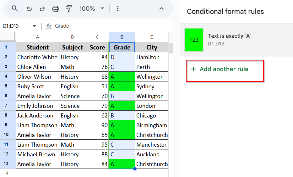
➤ Using the ‘Custom formula is’ function is a great way to add multiple conditions at once.
➤ You can add several built-in conditions simply by clicking the ‘add another rule’ option.
Using the AND Function
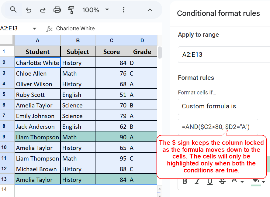
The AND function is one of the most commonly used functions for adding multiple conditions at once. When we use the AND function, the cells will be highlighted only when both conditions are met.
Let’s say we have a student score sheet, and we want to highlight the student rows who have both a score above 80 and an A grade. By using the AND function, this task will be very simple.
Here’s how you can do it:
Steps:
➤ Select all the rows containing data (A2:E13).
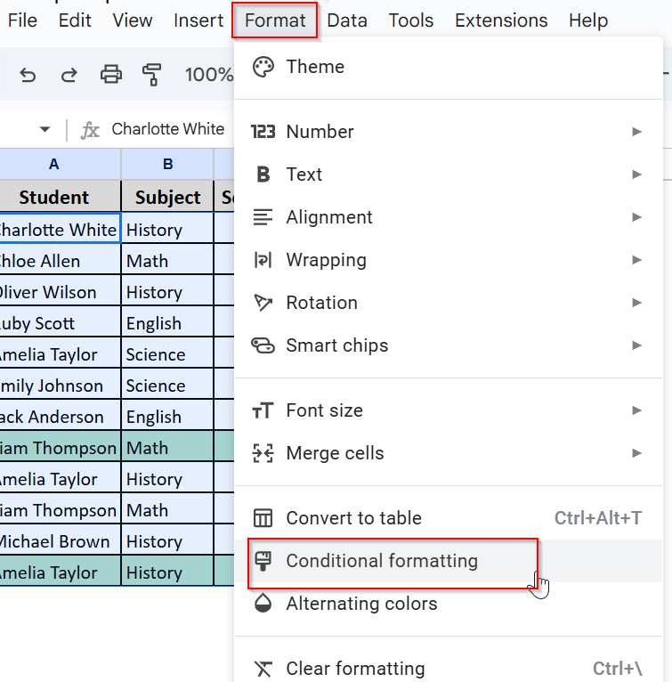
➤ Click on Format > Conditional Formatting.
➤ Choose Custom Formula is under the formatting rules
➤ Enter this formula:
=AND(C2>80, D2=”A”)
➤ Choose your preferred color
➤ Hit Done, and your cells are highlighted.
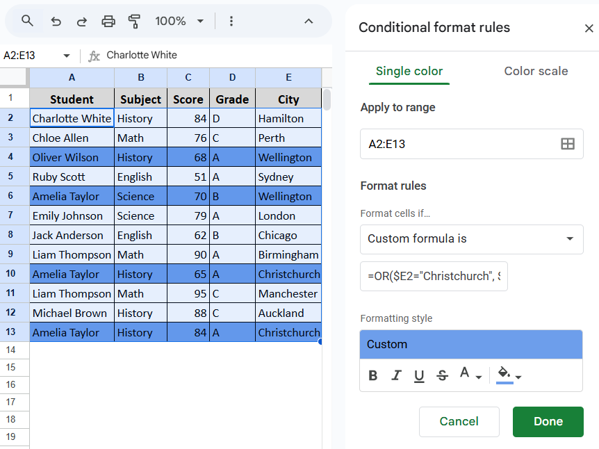
Using the OR Function
Highlight rows where the city is either “Christchurch” or “Wellington”. For that, we will again use the “conditional formula is” and the OR function. The OR function allows you to highlight cells when any one of the two conditions is met.
Here’s how you can do it:
Steps:
➤ Select the dataset from A2:E13.
➤ Go to Format > Conditional Formatting > Custom formula is.
➤ Type in this formula:
=OR(E2=”Christchurch”, E2=”Wellington”)
➤ Select your preferred color and click Done!
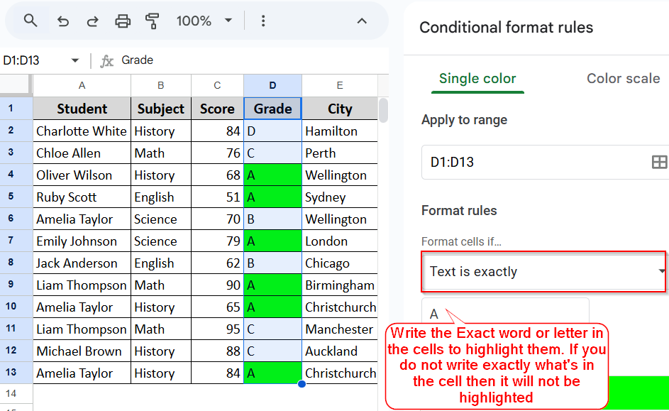
Applying Exact Match of the Text in the Condition
If you want to highlight all the grades and find students with higher or lower grades at once, using the Text is exactly condition in the formatting rule is a suitable option. The ‘text is exactly’ function finds the exact value you have given in the value box and highlights those cells.
Here’s how you can do it:
Steps:
➤ Select the Grades column to apply the formula to the grades.
➤ Go to Format > Conditional formatting
➤ Select Text is Exactly from the drop-down.
➤ Type in the Grade you want to highlight. I have written A in the value section because I want to highlight the A grades.
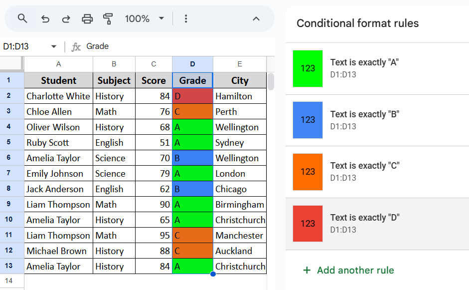
➤ As I want to highlight all the grades in different colors, I will add a few more conditions for each grade using the Text is Exactly function and change the grades in B, C, and D, respectively.
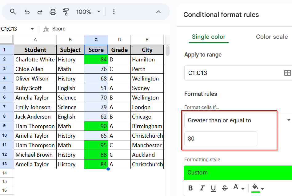
Using the Greater Than or Equal to Condition
This formatting rule will highlight all the scores above or equal to 80. This way, you can easily identify higher scores. Here’s how:
Steps:
➤ Select the Score column
➤ Go to Format > Conditional formatting.
➤ Select the Greater Than or Equal to formula.
➤ Enter 80 in the value section. You can change the value to your liking. I entered 80 to highlight cells with scores greater than or equal to 80.
➤ Click Done, and all the scores equal or above 80 will be highlighted.
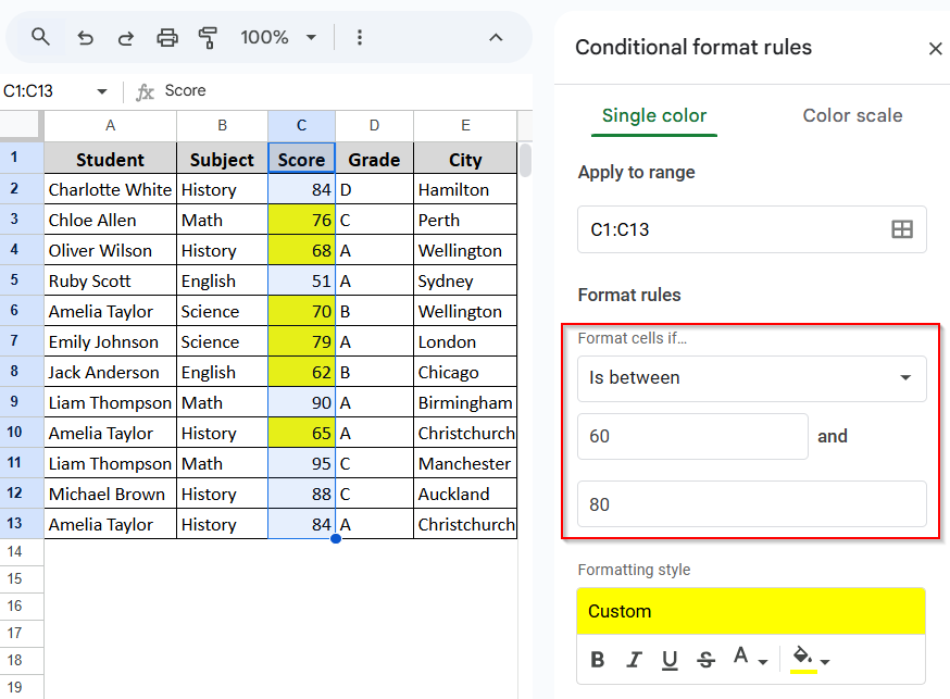
Using the Is Between Formatting Rule
What if you want to find students with scores between 60 and 80? That’s also very easy:
Steps:
➤ Go to the Conditional formatting and choose Is between.
➤ Enter the value of your choice. I have entered 60 and 80 to highlight the scores between 60 and 80.
➤ Hit Done and voila! Scores between 60 and 80 are highlighted.
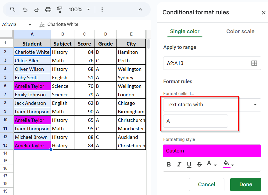
Using The Text Starts With Formula
Another very interesting formula is that text starts with. You can also find out the names of the students beginning with A. That is so easy!
Steps:
➤ Simply go to Conditional formatting.
➤ Choose text starting with a formula.
➤ Enter A (or any other letter you want).
➤ Click Done and that’s it!
Frequently Asked Questions (FAQs)
How does Google Sheets decide which color to show if two rules apply to the same cell?
Google Sheets applies rules in the order you create them. If two rules conflict, the later one usually takes priority. You can reorder rules in the conditional formatting pane to control which color appears.
Can I highlight an entire row based on a condition in one column?
Yes, you can format the entire row based on a specific condition by selecting the whole row range and using a custom formula that references the specific column with a dollar sign to fix it (e.g., $C2>80).
What should I do if my conditional formatting isn’t working as expected?
Check that your formula references match the top-left cell of your selected range and ensure there are no extra spaces or formatting issues in your data. Also, confirm that rules are applied to the correct range and order.
Concluding Words
Conditional formatting makes your sheets more organized and well-presented. Making the best use of Google Sheets starts with Conditional formatting. Once you master this function, there is no going back.
Although various built-in formulas exist, you can still enlarge your capacity with the custom formula option. Go through this article and get a grip on applying multiple functions. Feel free to reach out to us for any queries. We are always eager to hear from you.