When you have a lot of data in Google Sheets, it’s important to filter out duplicates so you don’t get the same value more than once. Duplicates can cause problems and make your analysis less accurate when you’re working with datasets like contact lists, survey responses, or product inventories. People usually look for this feature when they want to get rid of extra data, highlight unique entries, or make a report that doesn’t have any duplicates.
To filter out duplicates in Google Sheets, follow these steps:
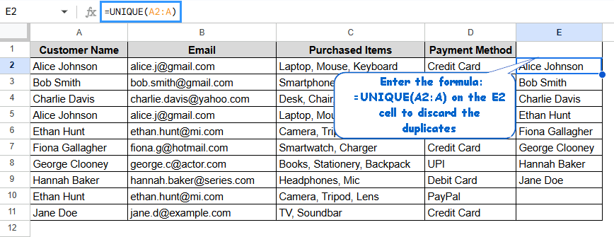
➤ Select an empty column, in this case E.
➤ Enter the formula:
=UNIQUE(A2:A)
➤ This will return a list of unique values and discard all duplicates. You can select all the columns and change the range.
We’ll look at different ways to filter out duplicates in Google Sheets in this article. Some of these are using built-in filter tools, conditional formulas, the UNIQUE function, and COUNTIF with helper columns. We’ll also talk about dynamic filtering with Apps Script and the Remove Duplicates Add-on for users who are more advanced.
What Is Duplicate Data in Google Sheets?
Duplicate data in Google Sheets can make it difficult to get accurate information and analyze it. It often happens because of mistakes made by people, problems with importing data, or wrong entries, which makes decisions less efficient and wastes resources. Common types of duplicate data are repeated rows or values, and each one needs a different way to be fixed.
To keep your data accurate and reliable, it’s important to get rid of duplicates in Google Sheets. Having duplicates can make mistakes, make bad decisions, and slow things down.
Using COUNTIF Function & Filter Tool to Identify Duplicates
This method is useful when you want to find duplicate entries without changing the original dataset. It’s especially helpful for finding duplicate entries in long lists, like names or emails of customers.
Steps:
➤ Select a new column, here column E.
➤ In the new column, enter the formula:
=COUNTIF(A:A, A2)>1
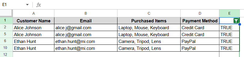
➤ This will return TRUE for duplicates and FALSE for unique values.
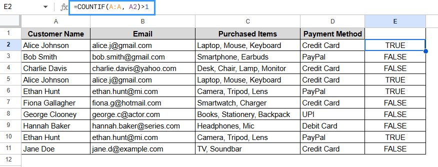
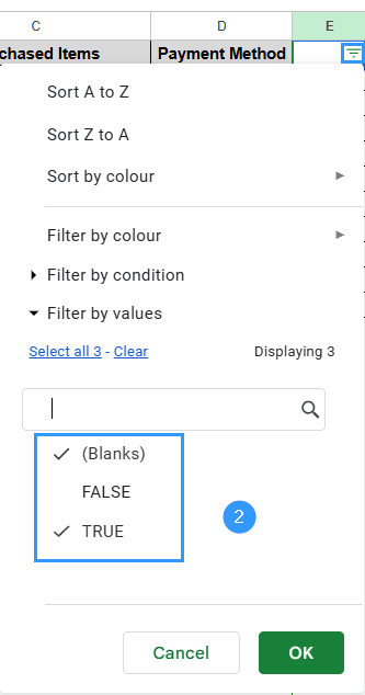
➤ Click Data > Create a Filter.

➤ Use the filter icon in the E column and select TRUE to show only the duplicate entries.
➤ You’ll see the result like this
Note:
If you want to highlight only the first instance of each duplicate, use:
=COUNTIF($A$2:A2, A2)>1
This highlights only repeated entries beyond the first.
Using the UNIQUE Function to Filter Duplicates
This method is great if you only want to show unique values from a column and get rid of duplicates automatically. It changes automatically when new data is added, which makes it great for connected sheets or live dashboards. This is a good way to make dropdowns or reports with filters.
Steps:
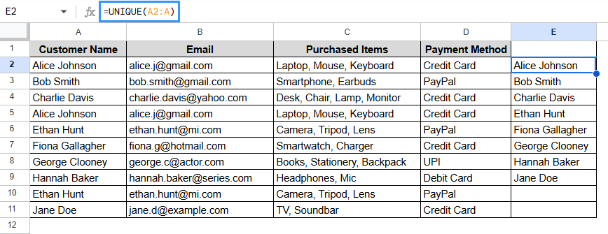
➤ Select an empty cell, here E2.
➤ Enter the formula:
=UNIQUE(A2:A)
➤ This process will return a list containing only the unique values, discarding any duplicates.
Note:
The UNIQUE function only shows unique values; it doesn’t change or hide the original dataset. UNIQUE doesn’t hurt your data; it only shows unique values in the output range, so your original data stays the same.
Using Conditional Formatting to Highlight Duplicates
Sometimes it’s better to just see where duplicates are instead of filtering. This method lets you quickly find duplicate entries without changing the way your data is set up. It’s especially helpful for going over data by hand or getting sheets ready for teamwork.
Steps:
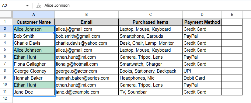
➤ Select the column you want to check for duplicates.
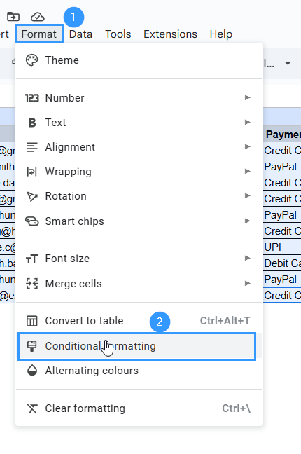
➤ Go to Format > Conditional formatting.
➤ Under the Format rules choose Custom formula.
➤ Enter the formula:
=COUNTIF(A:A, A1)>1
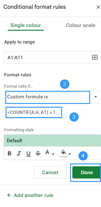
➤ You’ll see these results
Using Google Apps Script to Filter Duplicates Automatically
Apps Script can automatically filter out duplicates for users who work with large datasets that are always changing. You can use custom logic, like filtering based on certain columns or conditions. This method is excellent for automating routine data cleanup tasks that don’t require any work on your part.
Steps:
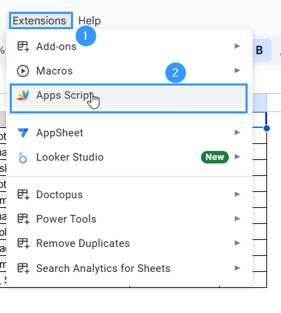
➤ Navigate to Extensions> Apps Script
 ➤ Save and Run the function by copying & then pasting the following code into the Apps Script editor.
function filterDuplicates() {
var sheet = SpreadsheetApp.getActiveSpreadsheet().getActiveSheet();
var data = sheet.getDataRange().getValues();
var seen = {};
for (var i = 1; i < data.length; i++) {
if (seen[data[i][0]]) {
sheet.hideRows(i + 1);
} else {
seen[data[i][0]] = true;
}
}
}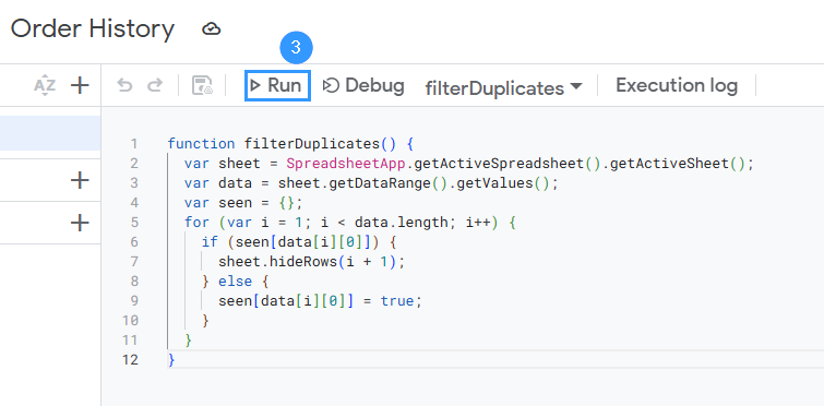
➤ This will hide duplicate rows based on the first column values. Here is the result

Note:
This only works on the first column. Modify data[i][0] to target other columns.
Frequently Asked Questions
What is the difference between filtering and removing duplicates in Google Sheets?
Filtering duplicates hides or separates repeated values so they can be seen or analyzed while removing duplicates permanently deletes them from the dataset.
How can I highlight only the second and onward duplicates?
Use this formula in conditional formatting:
=COUNTIF($A$2:A2, A2)>1
This will ignore the first one and highlight all the values that are the same.
Can I filter duplicates based on multiple columns?
Yes. If you want to combine conditions across more than one column, use COUNTIFS instead of COUNTIF:
=COUNTIFS(A:A, A2, B:B, B2)>1
Can I filter duplicates without using formulas?
Yes. You can find the Data menu and choose Data cleanup> Remove duplicates. This will remove duplicates instead of filtering them.
Can I keep one entry and hide the rest of the duplicates?
Yes. Use COUNTIF($A$2:A2, A2)=1 in a helper column, then filter for TRUE values to only show the first ones.
Concluding Words
One great way to clean up and organize your data in Google Sheets is to filter out duplicates. Removing or isolating duplicates helps make sure that datasets such as customer lists, inventory lists, or survey responses are all correct and clear. You can make your data workflow more efficient with built-in tools like conditional formatting and formulas like UNIQUE or FILTER, as well as Apps Script or add-ons for more experienced users.