

Manually separating numbers from texts from hundreds of rows is a tedious task no doubt. Unfortunately, Excel hasn’t yet developed any useful feature or direct function to do it quickly. To help you separate alphanumeric data, we’ve come up with multiple easy methods that anyone can follow.
You can quickly remove numbers from Excel cells using any of the effective methods given below:
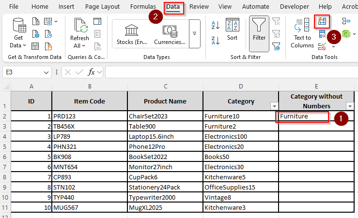
➤ Start by selecting a neighboring cell to the first data string of the column you want to delete numbers from. Type only the texts from the previous cell eliminating the numbers.
➤ Select and drag to highlight the new column. Press the keyboard shortcut CTRL + E to remove all numbers from the remaining text strings.
➤ Or, go to the Data tab, locate the Data Tools group on the top right corner of your screen, and click on the Flash Fill icon. Repeat the process for a second cell if it doesn’t work the first time.
Let’s dive into all the different ways of separating mixed text and numbers using simple features including Flash Fill and Power Query. We’ll also cover more complex methods such as using different array formulas and VBA coding.
Use the Flash Fill Feature for Patterned Data
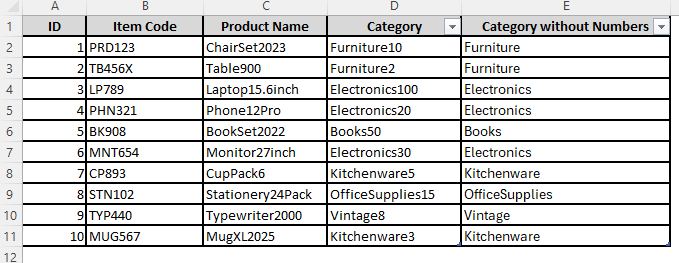
In this workbook, we created product datasets for a local shop with various product codes categories. We’ll work on the Category column where all the cells contain alphanumeric values. Our task is to keep the texts only and strip out the digits.
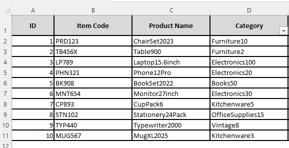
Excel typically identifies patterned data, so you can use the Flash Fill feature for text strings with numbers only on the right or left side. Let’s walk through the process.
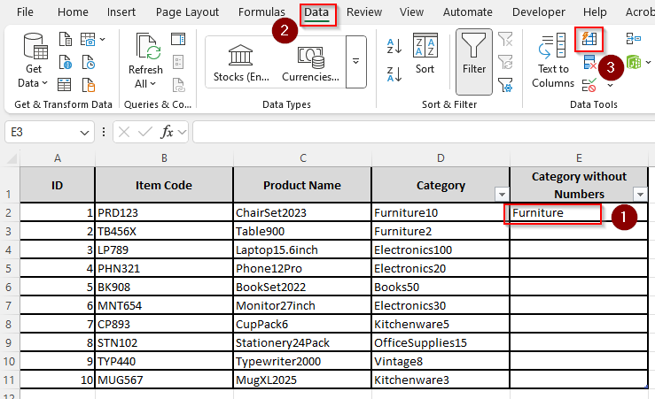
➤ Select the adjacent cell to your first text string and manually type the text from the first cell without the digits.
➤ For example, in the following pictures, cell D2 has the data string Furniture10. So, we entered Furniture in the E2 cell eliminating the numbers to help Excel recognize the pattern.
➤ Now, select the neighboring cell you’re using as an example, drag through the remaining cells of the column, and use the keyboard shortcut CTRL + E to apply the flash fill feature.
➤ You can also open the Data tab and click on the Flash Fill icon in the Data Tools group.
➤ As you can see, Excel has recognized the data pattern and omitted all numbers for each subsequent cell in the column.
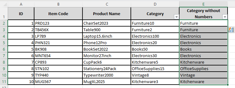
➤ If some of your cells have the correct text strings while others remain unchanged, you can fix this by taking another neighboring cell with uncorrected data and typing the correct text only without any numbers. Click Enter on your keyboard, and the remaining data will be sorted correctly.
Manually Remove Numbers with Find & Replace Tool
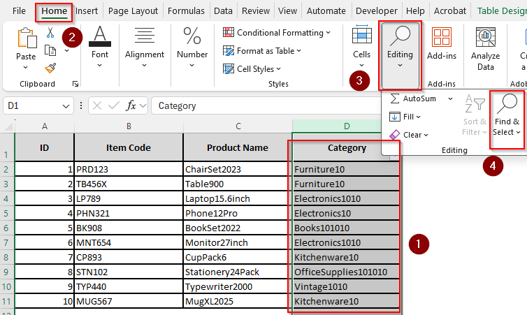
This method works when there are only common digits present in your dataset. To give you an example, we’ve changed the previous data to keep only the digits 1 and 0. For such less complex and small data sets, you can manually remove each number with the Find & Replace tool. Here’s how you can approach:
➤ Select the specific columns containing numeric data you want to change and use the shortcut CTRL + H to open the Find and Replace dialog box.
➤ Or, you can click on the Home tab. Press Find & Select from the Editing group on the top right corner of your screen.
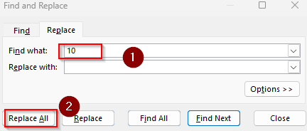
➤ In the Find and Replace dialog box, you need to type the exact digits you want to remove in the Find What box. We entered 10 in the box to get rid of all the numbers at once.
➤ Keep the Replace With box blank and click on Replace All.
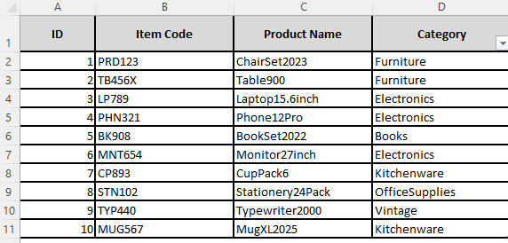
➤ In the following picture, Excel has removed all the zeros from our chosen column. If your data doesn’t have common digits, you need to repeat the process for all the remaining consecutive numbers from 1 to 9 putting only one digit at a time in the Find What box.
Replace Numbers with the SUBSTITUTE Function
Using the SUBSTITUTE function to replace all the digits with an empty string is a clever way to strip out numbers from texts. Here’s how to do it:
➤ Choose the adjacent cell to your first text string and type the following formula:
=SUBSTITUTE(SUBSTITUTE(SUBSTITUTE(SUBSTITUTE(SUBSTITUTE(SUBSTITUTE(SUBSTITUTE(SUBSTITUTE(SUBSTITUTE(SUBSTITUTE(D2,”0″,””),”1″,””),”2″,””),”3″,””),”4″,””),”5″,””),”6″,””),”7″,””),”8″,””),”9″,””)
➤ Replace D2 with the cell containing your text. Finally, choose the arrow icon and drag it until the last cell of the column containing your data.
The first function replaces 0 with an empty string, and the next one replaces 1 with an empty string within the result of the first. And this pattern continues for the remaining digits.
Apply Excel Formula with TEXTJOIN, ISNONTEXT, and MID Functions
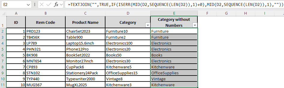
With this formula, we’ll use several functions to extract each character from a text string and then join only the non-numeric ones. Let’s proceed to the steps:
➤ In the neighboring cell of your preferred data cell, enter this formula:
=TEXTJOIN(“”,TRUE,IF(ISERR(MID(A1,SEQUENCE(LEN(A1)),1)+0),MID(A1,SEQUENCE(LEN(A1)),1),””))
➤ Instead of A1, type the actual reference of your data cell. Click on the arrow sign and drag it to select all the cells you want to convert.
REGEXREPLACE Function for Excel 365
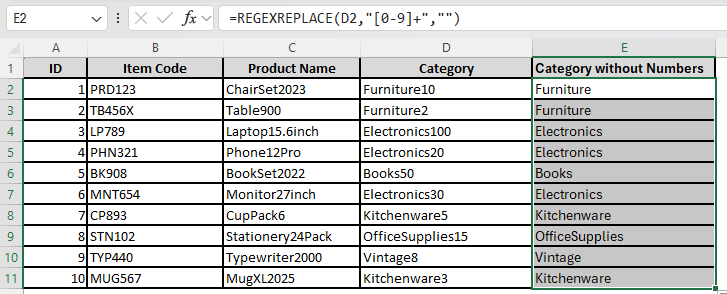
If you have Excel 365 or even a newer version featuring the REGEXREPLACE function, separating numbers from texts will take only a few clicks. Here’s how:
➤ Enter the following formula in your preferred cell and drag it down along the column with mixed alphanumeric data.
=REGEXREPLACE(A1,”[0-9]+”,””)
➤ Replace Cell A1 with the cell number of your preferred text string. This function locates all the digits from 0 to 9 expres to and replaces all occurrences of these digits with an empty string (“”).
Enter an Array Formula to Extract Text
With proper knowledge of how Excel formulas work, one can create a detailed formula to filter texts from mixed alphanumeric data. Here, we’ll use such an array formula that you can simply copy and paste to quickly get the job done. Follow the steps given below:
➤ Select the adjacent cell to the first text string of the column you want to convert. Start typing the following formula and press Enter:
=CONCAT(FILTER(MID(D2,SEQUENCE(LEN(D2)),1),ISERROR(MID(D2,SEQUENCE(LEN(D2)),1)*1)))
➤ Always use the exact cell reference of your chosen column cell in the formula instead of D2.
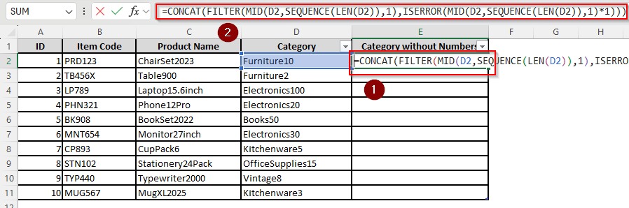
➤ Click and drag the formula until the last row of your data to remove all the digits from your data sets.
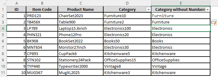
Finally, we use a FILTER that keeps only the characters where ISERROR is TRUE (text in this case). CONCAT is used to join our filtered texts in a string.
Remove Digits Using the Power Query Feature
Before getting into more complicated formulas, let’s try the Power Query feature. It’s a powerful transformation feature that allows you to customize worksheet columns in your preferred ways. Start by following these steps:
➤ Drag and select the column you want to transform and go to the Data tab. Navigate to the Get & Transform Data group and select Get Data. Click on From Other Sources and choose From Table/Range.
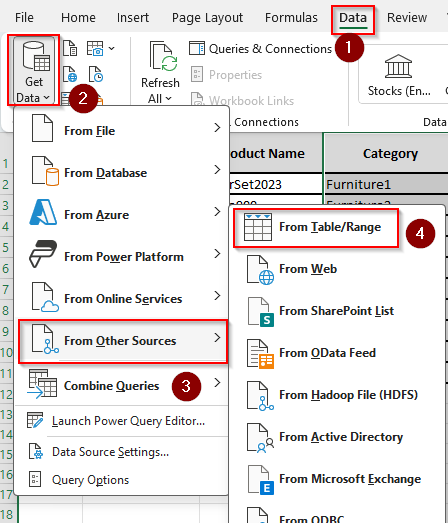
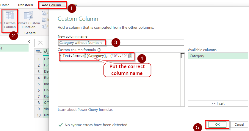
➤ As the Power Query Editor arrives, press on the Add Column tab and select Custom Column.
➤ In the New Column Name field, add a name if you like. Proceed to the Custom Column Formula box and type either of the following formulas
- Remove([ColumnHeading], {“0”..”9″})
- Select([ColumnHeading], {“A”..”Z”, “a”..”z”})
➤ You must replace ColumnHeading with the actual name of the column you’re extracting text from. As you can see in the picture, we replaced ColumnHeading with Column without Numbers.
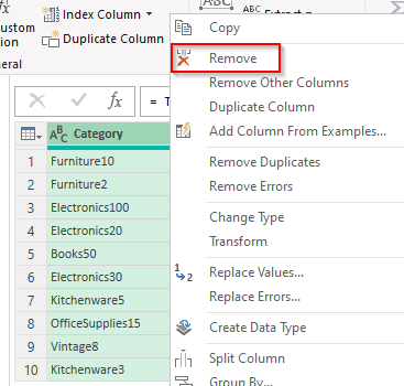
➤ To avoid creating a copy of the source column, right-click on the source column and select Remove.
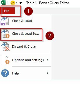
➤ Go to File and choose Close & Load To…
➤ From the Import Data dialog box, select Table and Existing Worksheet. Use the arrow sign to select a new column in your worksheet where you want to store the converted data.
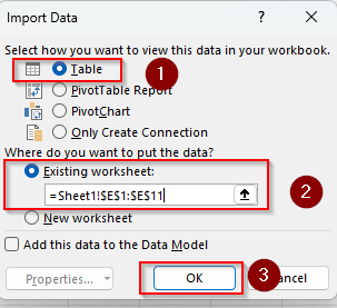
➤ Finally, click Ok to create a new column with only texts as shown below:
Eliminate Numbers with VBA Coding
With VBA macros, you can remove numbers from longer and more complex data sets. However, you need to enter a custom function first. So, follow the steps given below:
➤ Open the VBA Editor by pressing the keyboard shortcut Alt + F11 . You can also go to the Developer tab and select Visual Basic.
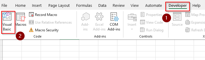
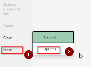
➤ If you don’t have the Developer tab on the main ribbon, go to the File tab, click on More, and select Options.
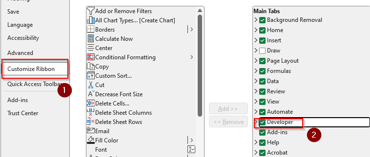
➤ Go to Customize Ribbon and check the Developer box from the Main Tabs group. Click Ok.
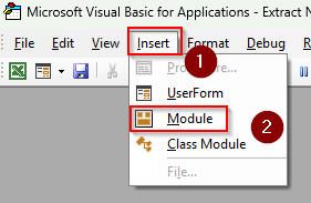
➤ In the VBA editor, go to Insert, select Module, and paste either of the following codes:
To Keep Texts Only and Remove the Numbers Completely
Sub KeepOnlyText()
' This macro removes all numeric characters from the selected cell(s),
' leaving only the text.  It handles spaces and other non-numeric characters.
  Dim cell As Range
  Dim inputRange As Range
  Dim textString As String
  Dim i As Long
  Dim character As String
  ' Get the user's input range.  Error handling is important.
  On Error Resume Next
  Set inputRange = Application.InputBox( _
    Prompt:="Select the range of cells to process (text will be kept, numbers removed):", _
    Title:="Select Range", _
    Type:=8) ' Type 8 for range selection
  On Error GoTo 0
  ' Exit if the user cancelled.
  If inputRange Is Nothing Then
    MsgBox "No range was selected. Exiting.", vbExclamation
    Exit Sub
  End If
  ' Disable screen updating for efficiency.
  Application.ScreenUpdating = False
  ' Loop through each cell in the selected range.
  For Each cell In inputRange
    textString = "" ' Reset the string for each cell.
    ' Loop through each character in the cell's value.
    For i = 1 To Len(cell.Value)
      character = Mid(cell.Value, i, 1)
      ' Check if the character is NOT numeric.  If it's not, keep it.
      If Not IsNumeric(character) Then
        textString = textString & character
      End If
    Next i
    ' Put the resulting text back into the cell.
    cell.Value = textString
  Next cell
  ' Re-enable screen updating.
  Application.ScreenUpdating = True
  ' Inform the user that the process is complete.
  MsgBox "Numbers removed, text kept!", vbInformation, "Done!"
End Sub
To Put Text and Numbers in Separate Columns
Sub SeparateTextAndNumbers()
  ' This macro separates text and numbers from a selected range of cells.
  ' It places the text in the adjacent column to the right, and the numbers
  ' in the column next to that.
  Dim cell As Range
  Dim inputRange As Range  ' Changed variable name for clarity
  Dim textString As String
  Dim numberString As String
  Dim i As Long
  Dim character As String
  Dim lastRow As Long
  ' Error handling in case no range is selected.
  On Error Resume Next
  Set inputRange = Application.InputBox( _
    Prompt:="Select the range of cells to process:", _
    Title:="Select Range", _
    Type:=8) ' Type 8 is for selecting a range
  On Error GoTo 0
  ' Exit if no range was selected
  If inputRange Is Nothing Then
    MsgBox "No range was selected.  Exiting.", vbExclamation
    Exit Sub
  End If
  ' Disable screen updating to speed up processing
  Application.ScreenUpdating = False
  ' Loop through each cell in the selected range
  For Each cell In inputRange
    textString = ""
    numberString = ""
    ' Loop through each character in the cell's value
    For i = 1 To Len(cell.Value)
      character = Mid(cell.Value, i, 1) ' Get one character at a time
      ' Check if the character is a number (and not a space).
      '  IsNumeric(" ") returns True, so we exclude spaces.
      If IsNumeric(character) And character <> " " Then
        numberString = numberString & character
      Else
        textString = textString & character
      End If
    Next i ' Go to the next character
    ' Write the results to the adjacent cells.  Using Offset is good.
    cell.Offset(0, 1).Value = Trim(textString)      ' Text to the right
    cell.Offset(0, 2).Value = numberString    ' Numbers to the right of the text
  Next cell ' Go to the next cell in the selected range
  ' Re-enable screen updating
  Application.ScreenUpdating = True
  ' Show a message when done.
  MsgBox "Text and numbers separated successfully!", vbInformation, "Done!"
End Sub
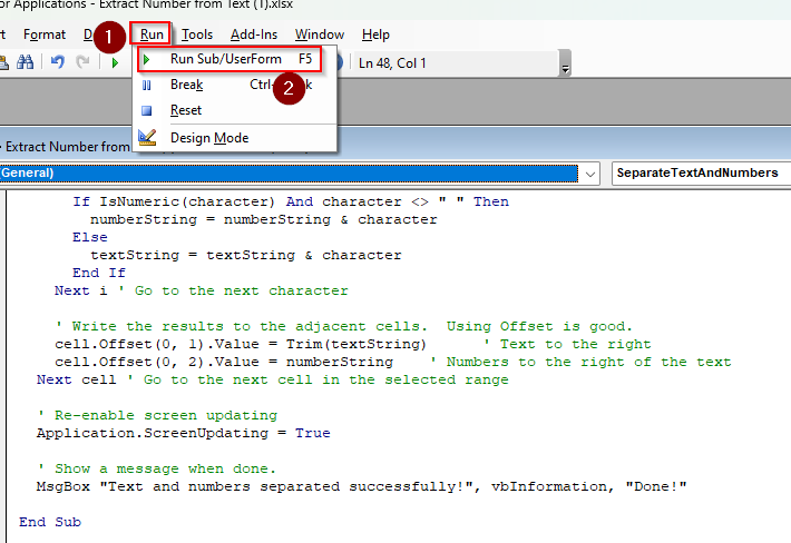
➤ Click on the Run tab and select Run Sub/UserForm.
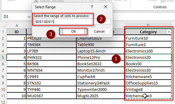
➤ Now, in the new dialog box, you need to type the column range where you want to apply the VBA macro.
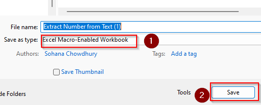
➤ To save the changes, go to File and go to Save As. Navigate the location where you want to save the workbook. In the Save as Type box, choose Excel Macro-Enabled Workbook and press Save.
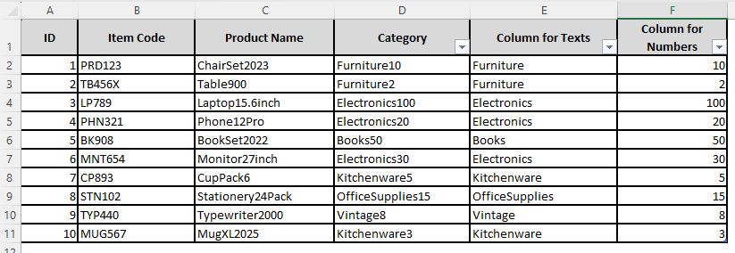
➤ Here’s the final result for the second code:
Downloadable Resources
Get our practice workbook or necessary files that we have worked with to prepare this article.
Remove Numbers from a Cell.zip
Frequently Asked Questions
How do I remove 3 digits from the left in Excel?
You can use the RIGHT and LEN functions to create a formula that removes 3 digits from the left side of a text string. Select the cell and type:
=RIGHT(A1, LEN(A1)-3)
If you want to remove more than 3 digits put the exact number of digits instead of 3 in the formula. Replace the RIGHT function with LEFT to remove 3 digits from the left side of the cell.
How to take only numbers from a cell in Excel?
Select your preferred column and go to the Data tab >> Get Data >> From Other Sources >> From Table/Range. Use the Power Query feature to create a custom column and enter the formula:
Text.Remove([ColumnHeading], {“A”..”Z”, “a”..”z”})
How to remove delimited numbers from text?
If the digits in your columns are separated by delimiters such as comma, tab, semicolon, plus sign, space, or hyphen, use the Text to Columns feature you can find on the Data tab. As the Text Import Wizard box arrives, click on Delimited and choose the right delimiter from the options. If the delimiter of your data feature isn’t in the list, manually type it in the Other box. Finally, choose General and click Finish.
Wrapping Up
All the methods we’ve mentioned to separate numbers from text are roundabout ways that might take several trial and error. If your data sheet is long and complex, use the array formulas or VBA macros for accurate results.
To finish the task easily in just a few clicks, the Flash Fill feature is preferable for small data sets. There are other more complicated ways to do the task such as using third-party add-ins. However, these can be harmful for your device.