When working with large datasets in Google Sheets, summarizing data by categories, like totals by region or averages by product, is essential for analysis. The QUERY function, which uses a SQL-like syntax, lets you group data effortlessly using the GROUP BY clause. Whether you’re calculating totals, averages, counts, or other aggregate values, this method keeps your reports clean and dynamic.
In this article, we’ll explore how to use the QUERY function with GROUP BY to organize and summarize data efficiently, using a sample dataset of regional sales.
Steps to summarize the total using QUERY and GROUP BY functions:
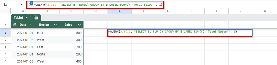
➤ Click on a blank cell (e.g., E2) where you want the summary table to appear.
➤ Type the following formula:
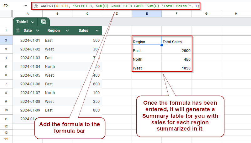
=QUERY(A1:C11, “SELECT B, SUM(C) GROUP BY B LABEL SUM(C) ‘Total Sales'”, 1)
➤ Press Enter.
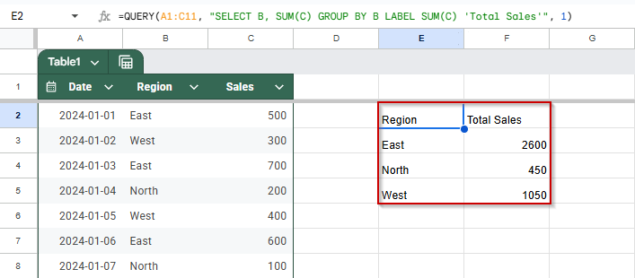
Summarize Total Value Using QUERY with GROUP BY
Use this method when you want to quickly calculate the total sales for each region from your dataset. It’s perfect for generating summary reports where data is grouped by category and totaled using the QUERY function in Google Sheets.
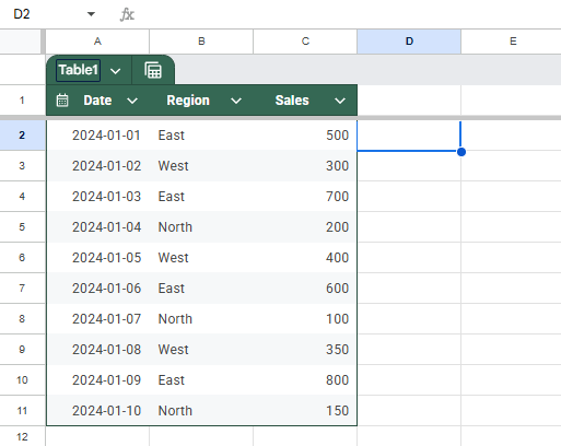
We’ll use the following sample dataset in A1:C11, where column B contains regions and column C contains sales figures:
Steps:
➤ Click on a blank cell (e.g., E2) where you want the summary table to appear.
➤ Type the following formula:
=QUERY(A1:C11, “SELECT B, SUM(C) GROUP BY B LABEL SUM(C) ‘Total Sales'”, 1)
➤ Press Enter.
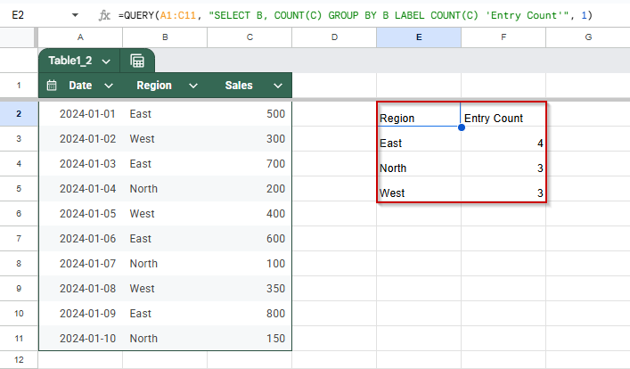
QUERY with GROUP BY to Count Entries
Use this method when you want to count how many sales records exist for each region in your dataset. This is useful for understanding how frequently each region appears, regardless of sales amount, using the QUERY function with COUNT and GROUP BY functions.
We’re using the same dataset in A1:C11, where column B contains the region names and column C contains sales figures.
Steps:
➤ Click on a blank cell (e.g., E2) where you want the summary to appear.
➤ Type the following formula:
=QUERY(A1:C11, “SELECT B, COUNT(C) GROUP BY B LABEL COUNT(C) ‘Entry Count'”, 1)
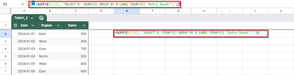
➤ Press Enter.
QUERY with GROUP BY to Calculate Average in Google Sheets
Use this method to find the average sales amount for each region in your dataset. It’s helpful for identifying which regions consistently perform better or worse on average, regardless of how many sales entries they have. We’ll use the QUERY function with AVG() and GROUP BY for this calculation.
Steps:
➤ Click on a blank cell (e.g., E2) where you want the result to appear.
➤ Type the following formula:
=QUERY(A1:C11, “SELECT B, AVG(C) GROUP BY B LABEL AVG(C) ‘Average Sales'”, 1)
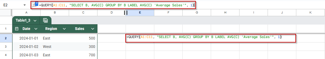
➤ Press Enter.
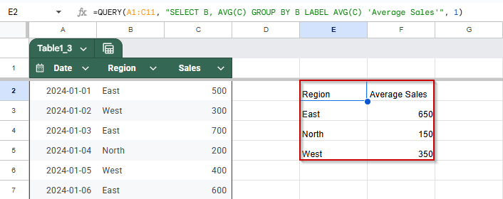
This formula groups all rows by region and calculates the average value from the Sales column for each region. The result will display one row per region with its corresponding average sales figure.
Frequently Asked Questions
What is the purpose of the GROUP BY clause in Google Sheets QUERY?
The GROUP BY clause aggregates data based on specified columns, allowing you to summarize information like totals or averages for each group in your dataset.
Can I group data by multiple columns in a QUERY function?
Yes, you can group by multiple columns by listing them in the GROUP BY clause, enabling multi-level data aggregation for more detailed summaries.
What aggregate functions can be used with GROUP BY in QUERY?
Common aggregate functions include SUM, COUNT, AVG, MIN, and MAX, which calculate totals, counts, averages, minimums, and maximums within each group.
How do I sort grouped data in QUERY results?
Use the ORDER BY clause after GROUP BY to sort the results based on a specific column, either in ascending (ASC) or descending (DESC) order.
Wrapping Up
Using the GROUP BY clause in the Google Sheets QUERY function is a powerful way to summarize your data. Whether you’re tallying sales totals, counting entries, or calculating averages by category, GROUP BY helps transform raw rows into meaningful insights. With just a few lines of formula, you can automate your reports and make your data easier to analyze at a glance.