
Sometimes you need to combine data from multiple cells in Google Sheets, but the regular Merge option just keeps the top-left value and drops everything else.
That’s not ideal when you want to keep all your information in one place.
For example, maybe you want to join a first and last name, or combine a few values into a single line for a report. There are a few easy ways to do this without losing anything.
➤ Click on the cell where you want to show the merged result.
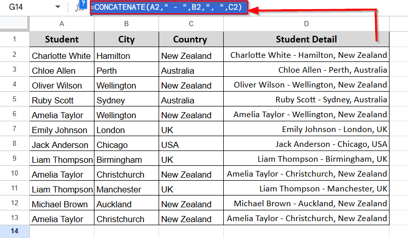
➤ Enter the formula: =CONCATENATE(A2, ” – “, B2, “ , “,C2)
➤ Replace A2, B2, and C2 with any other cells you want to merge.
➤ Add a space, comma, string, or any symbol inside the quotes if you want separation between values.
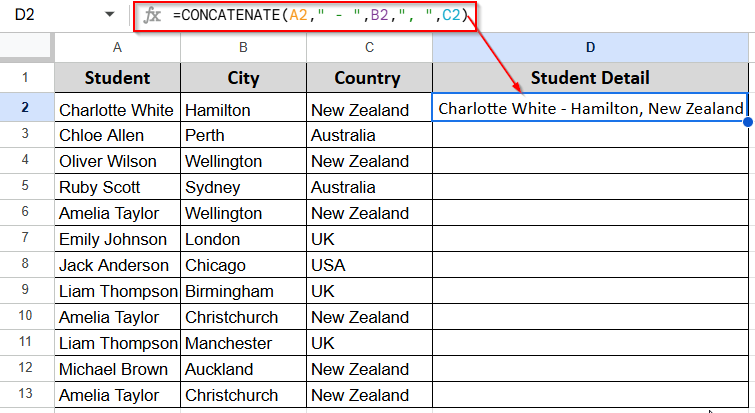
➤ Press Enter to see the combined result in one cell. In this case, it is D2.
➤ After pressing Enter, use the Fill Handle tool to copy the formula down the column.
Apply CONCATENATE Function
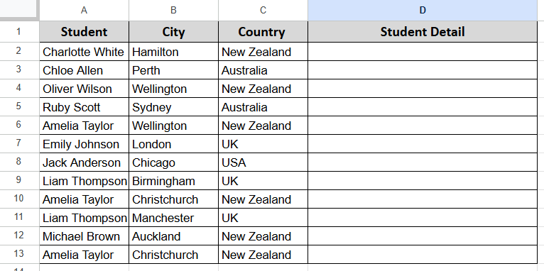
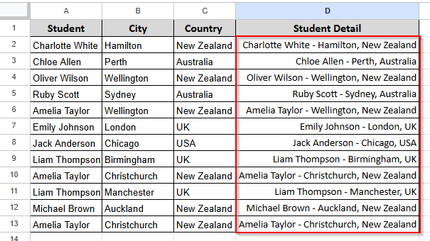
In the following dataset, we have the names of students in Column A, their cities in Column B, and the corresponding countries listed in Column C.
Our goal is to merge data from the columns A, B, and C into column D without losing any data.
Let’s use the CONCATENATE function to merge the student’s name, city, and country into one cell with separators.
Steps:
➤ Select the output cell (D2) and insert the following formula.
=CONCATENATE(A2,” – “,B2,”, “,C2)
Note:
You can use empty space or any other string inside double quotes, and the output will show the strings.
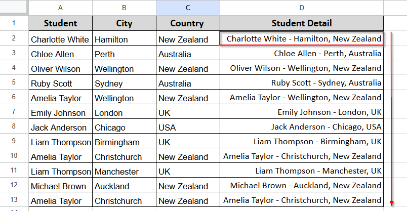
➤ After pressing the Enter button, use the Fill Handle tool to apply the formula down the column for the remaining rows.
Note:
The CONCATENATE function works well when you’re combining a few specific cells. But it doesn’t support ranges or ignore empty cells. If your data has missing values or you need to combine a larger set of cells, try using the TEXTJOIN function instead. It’s more flexible for those cases.
Using JOIN Function to Merge Cells without Losing Data
In the following dataset, we have the names of students in Column A. The cities they have visited are listed across Columns B, C, and D.
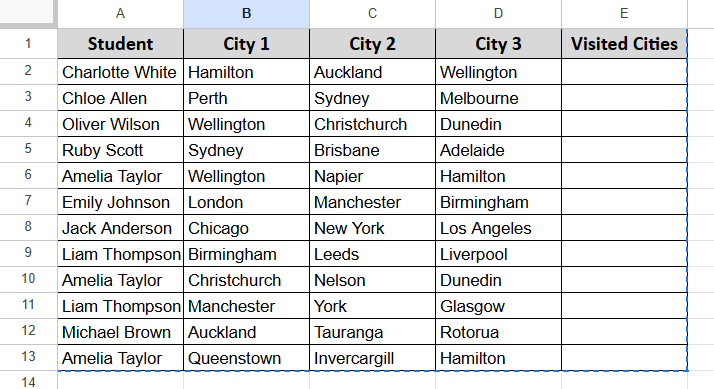
Let’s use the JOIN function to combine all visited cities into a single cell for each student. We’ll separate the cities using commas.
Steps:
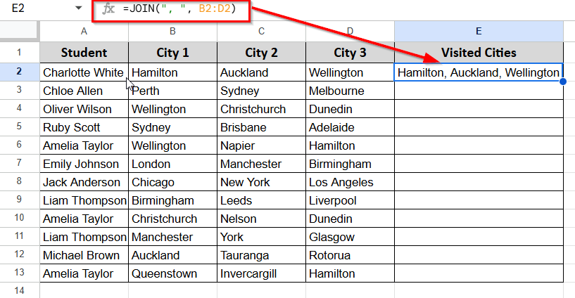
➤ Select the output cell (E2) and insert the following formula.
=JOIN(“, “, B2:D2)
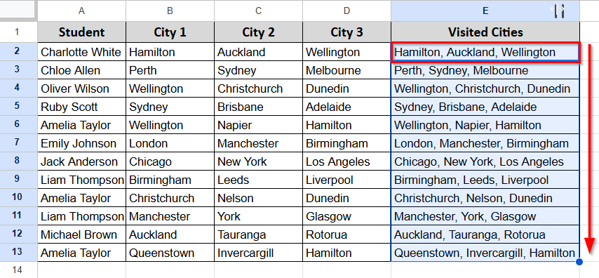
➤ After pressing the Enter button, use the Fill Handle tool to copy the formula down the column for the rest of the students.
Note:
The JOIN function works well when all the cells in the range have values. But if any of the cells are blank, it still includes extra separators. If you want to skip blanks automatically, the TEXTJOIN function handles that better.
Insert the TEXTJOIN Function to Merge Cells
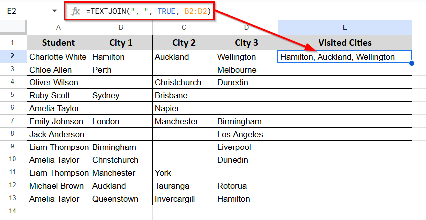
In the following dataset, we have the names of students in Column A. Their visited cities are listed in Columns B, C, and D. Some students have visited fewer than three cities, so a few cells are blank.
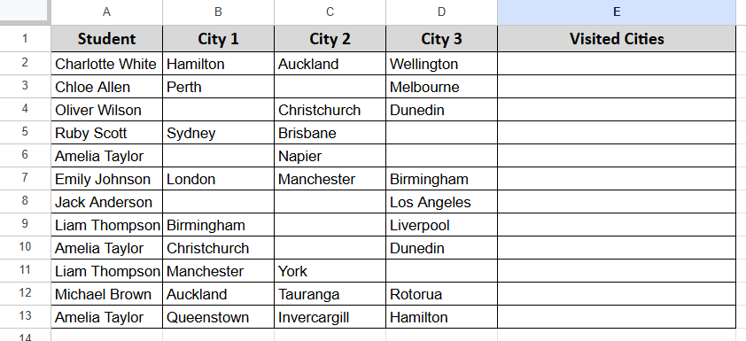
Let’s use the TEXTJOIN function to combine all the visited cities into a single cell. This function skips over empty cells automatically. So, it’s pretty handy when you have messed up data.
Steps:
➤ Select the output cell (E2) and insert the following formula.
=TEXTJOIN(“, “, TRUE, B2:D2)
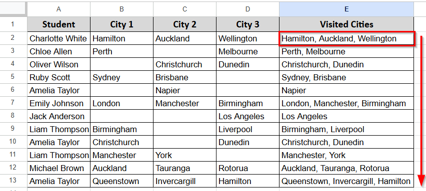
➤ After pressing the Enter button, use the Fill Handle to apply the formula to the rest of the rows.
Note:
TEXTJOIN is great when your data isn’t perfectly filled in. It automatically skips over any blanks, so you don’t get extra commas or awkward spaces in your results.
Using Ampersand (&) Operator to Combine Cells
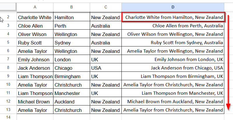
In the following dataset, we have student names in Column A, their cities in Column B, and countries in Column C. We’ll use the Ampersand operator (&) to combine these values into a single line of text.
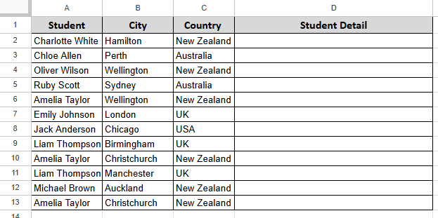
Let’s use the Ampersand to create a readable sentence that includes the name, city, and country of each student.
Steps:
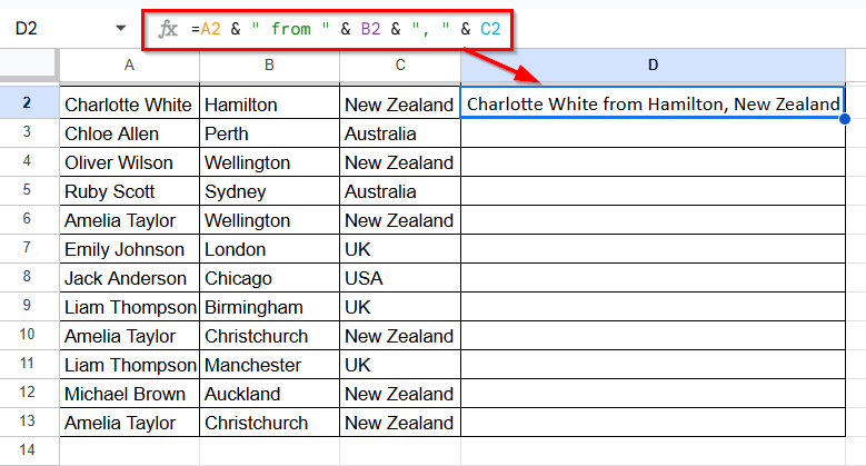
➤ Select the output cell (D2) and insert the following formula.
=A2 & ” from ” & B2 & “, ” & C2
➤ After pressing Enter, drag the Fill Handle to apply the formula to the rest of the rows.
Note:
The Ampersand (&) lets you join cells quickly and gives you more control over the format. It’s easier to read and write than CONCATENATE, especially for short, custom outputs.
Apply CHAR(10) Function
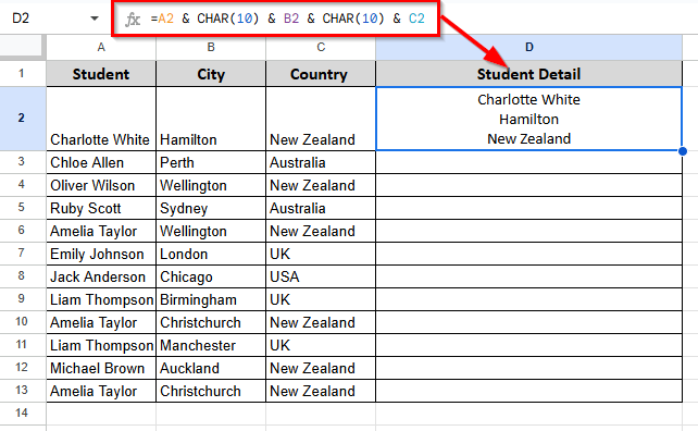
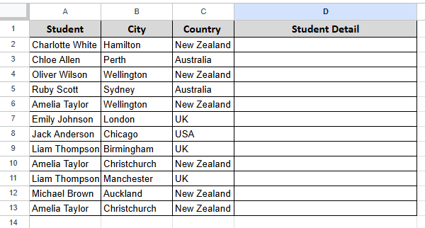
In the following dataset, we have student names in Column A, their cities in Column B, and countries in Column C.
Now we’ll use the CHAR(10) function to add line breaks inside a single cell, so each piece of information appears on a separate line.
Let’s use the Ampersand symbol with CHAR(10) to combine name, city, and country in one cell—each on its own line.
Steps:
➤ Select the output cell (D2) and insert the following formula.
=A2 & CHAR(10) & B2 & CHAR(10) & C2
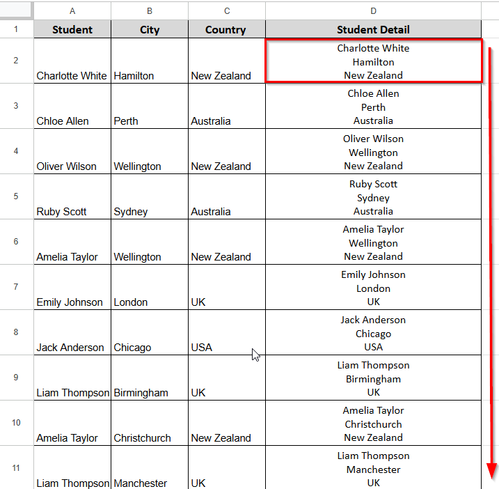
➤ After pressing Enter, make sure to enable “Wrap Text” for Column D so the line breaks are visible. Then, use the Fill Handle to apply the formula to the other rows.
Note:
CHAR(10) works only when Wrap Text is turned on. Otherwise, the result will look like a single line with weird spacing.
Merge Cells Using Google Apps Script
If you’re tired of dragging formulas down every time you update your sheet, this one’s for you. Apps Script lets you run a bit of code that does the merging for you. It’s built right into Google Sheets, so you don’t need anything extra.
We’ll work with data in Columns A, B, and C—student name, city, and country. Our goal is to put all of that into Column D in this format:
Steps:
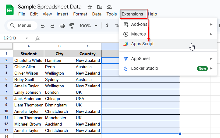
➤ Go to Extensions and open Apps Script.
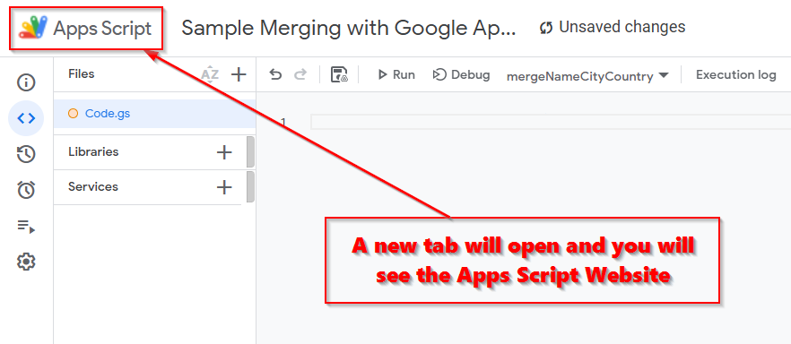
➤ A new tab will open, and you will see this page
➤ Delete the default function if there’s one.
➤ It’ll ask you to name the project. You can type something simple like “MergeDataScript”. Giving it a name helps you find it later if you create more scripts in the same file. In our case, we named it “Sample Merging with Google App Script”

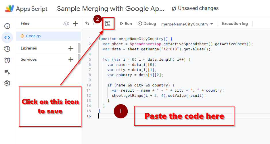
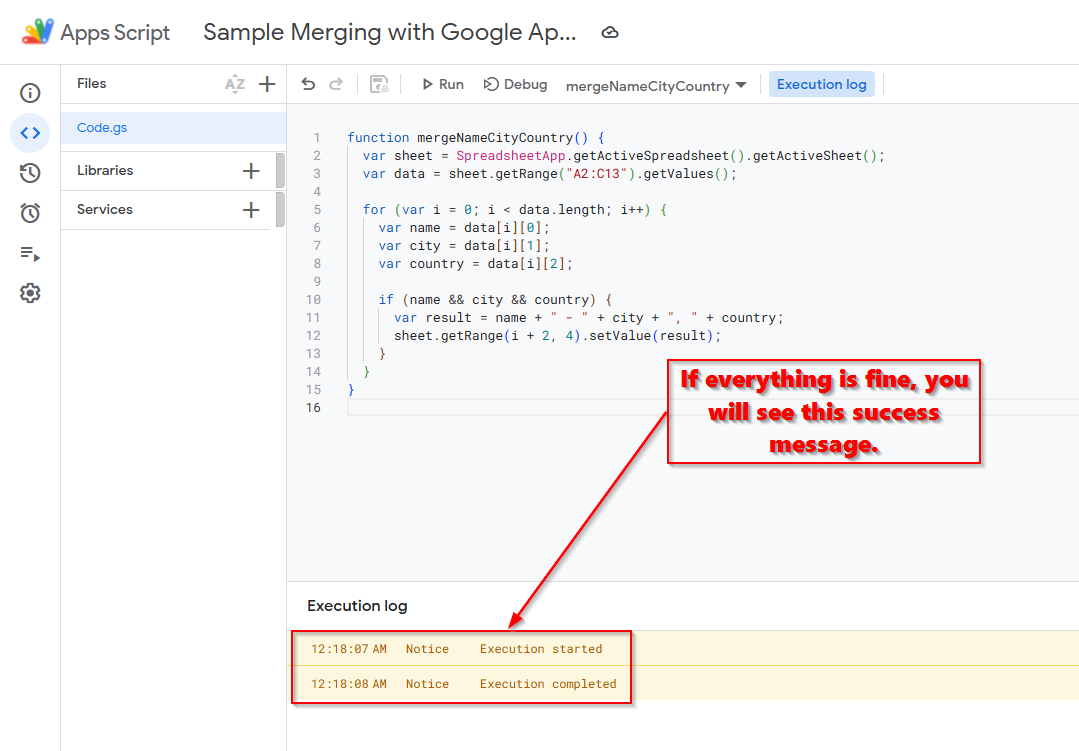
➤ Paste this code:
function mergeNameCityCountry() {
  var sheet = SpreadsheetApp.getActiveSpreadsheet().getActiveSheet();
  var data = sheet.getRange("A2:C13").getValues();
  for (var i = 0; i < data.length; i++) {
    var name = data[i][0];
    var city = data[i][1];
    var country = data[i][2];
    if (name && city && country) {
      var result = name + " - " + city + ", " + country;
      sheet.getRange(i + 2, 4).setValue(result);
    }
  }
}
➤ Save the script by clicking the small disk icon.
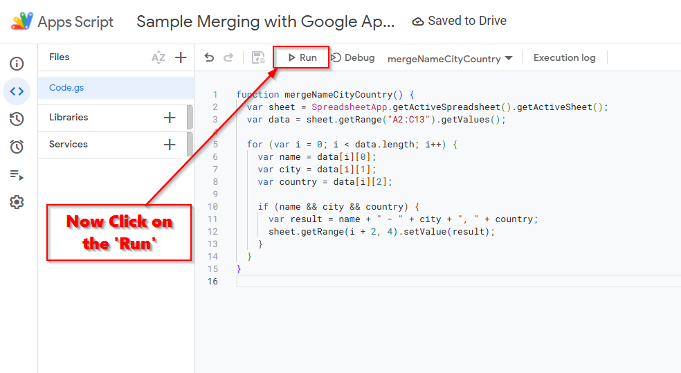
➤ Then press Run. It’ll ask for permission the first time—just go ahead and allow.
➤ You will see the success message
➤ Now go to your Google sheet and you will see the merged data in the Student Detail column (D). You don’t need to use the Fill Handle option because all the rows are already filled with data.
Note:
If your data goes beyond Row 13, change the range “A2:C13” to match the size of your sheet. For example, if you have 200 rows, use “A2:C201“.
Frequently Asked Questions
Why does sorting stop working when I merge cells?
It’s just how Sheets handles it. If even one cell in the range is merged, the whole sort can fail or go weird. Try to leave your sorting areas untouched—no merging there.
Can I freeze merged rows or columns?
Not really. Google Sheets doesn’t handle that well. You might be able to do it in parts, but it won’t behave right.
What happens when I unmerge something?
Only the top-left part stays. Everything else just disappears. So, copy the data somewhere else.
Concluding Words
Merging can be handy, but only if it fits your goal. Pick the method that suits what you’re trying to do. In this article, we described 5 processes to merge cells in Google Sheets without losing data. We suggest that you learn all methods so that you can pick one that will help you save time and do the job efficiently. Last of all, always back up your data before merging. If anything goes wrong, you can always start over from that backup.