
Data validation in Google Sheets is a very important skill. For example, you are making a sheet where users will insert business email addresses, but some people are writing without “@” or adding non-business emails.
If you apply the right data validation rule, Google Sheets will block that kind of input and give a warning message to the person who is doing the job.
In this article, we’ll talk about 5 widely used methods with specific use cases. Let’s explore them.
➤ Select the range D2:D13 where you want to apply data validation rules.
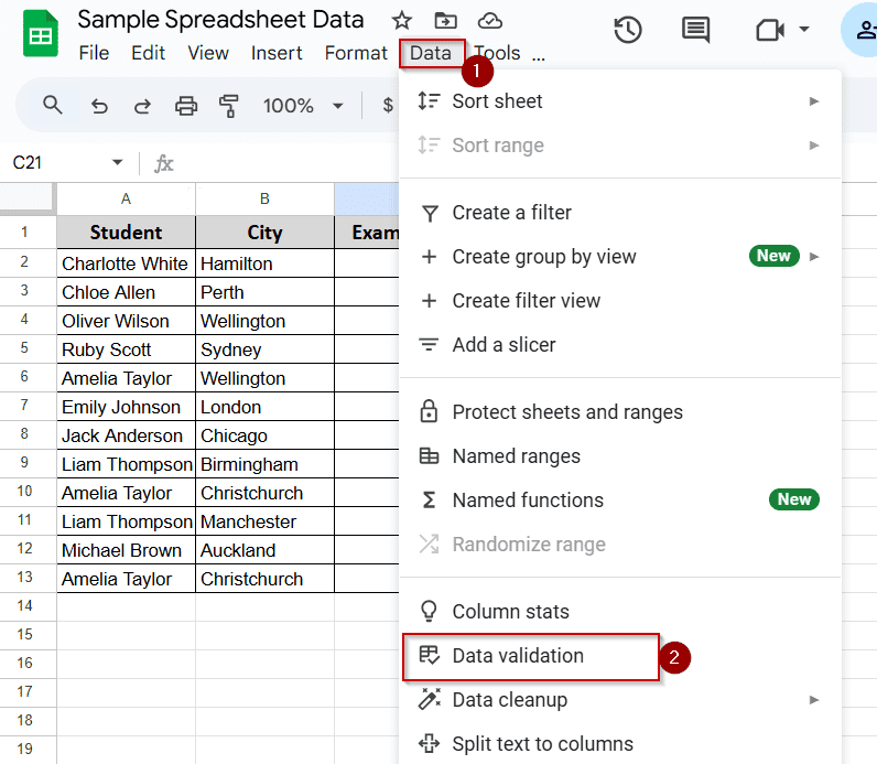
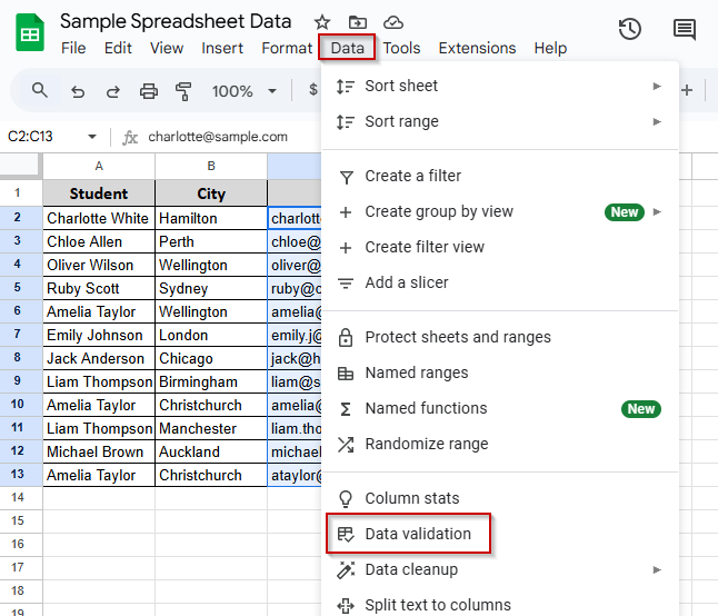
➤ Go to Data > Data validation (From the Menu Bar)
➤ Set criteria to “Custom formula is”
➤ We want the exam score column to take data between 40 and 100 only.
➤ Enter this formula: =AND(ISNUMBER(D2), D2>=40, D2<=100)
➤ Now Column D won’t take any number that is not within this range.
➤ To give a warning, you can click on Advanced Options and write “Number should be between 40 and 100,” and users will see this error if they insert a number outside this range.
➤ Click on “Done.”
➤ You can see red marks at the top right corner of those numbers that are under 40.
Number Range Validation
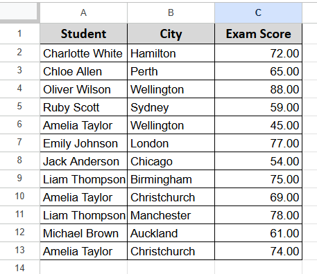
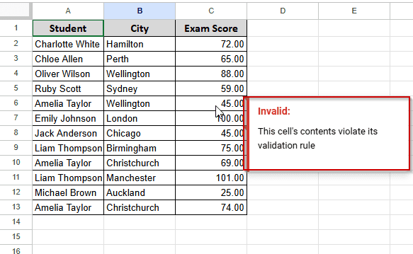
In the following dataset, we have a list of students in Column A and their cities in Column B. In the third column (Column C), we’ve their Exam Score.
We want to make sure the values in the Exam Score column stay between 40 and 100. So, if anyone inserts data can’t add any data outside of this range.
Let’s begin.
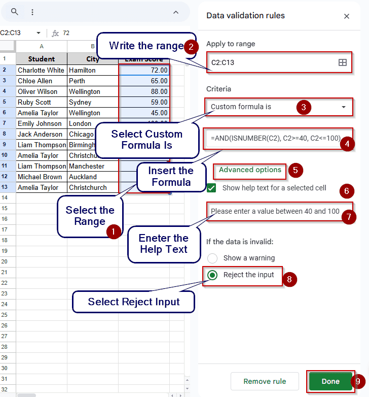
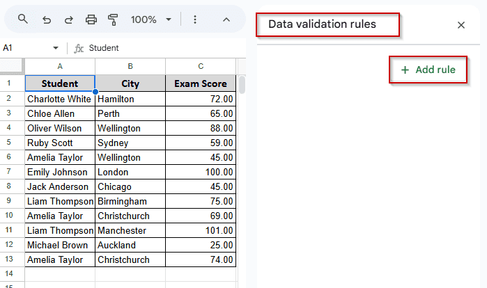
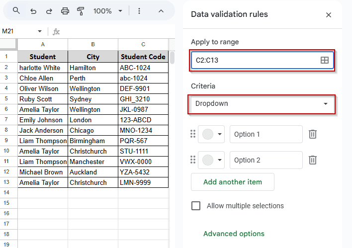
➤ Select the Exam Score cells. In this case, from C2 to C13.
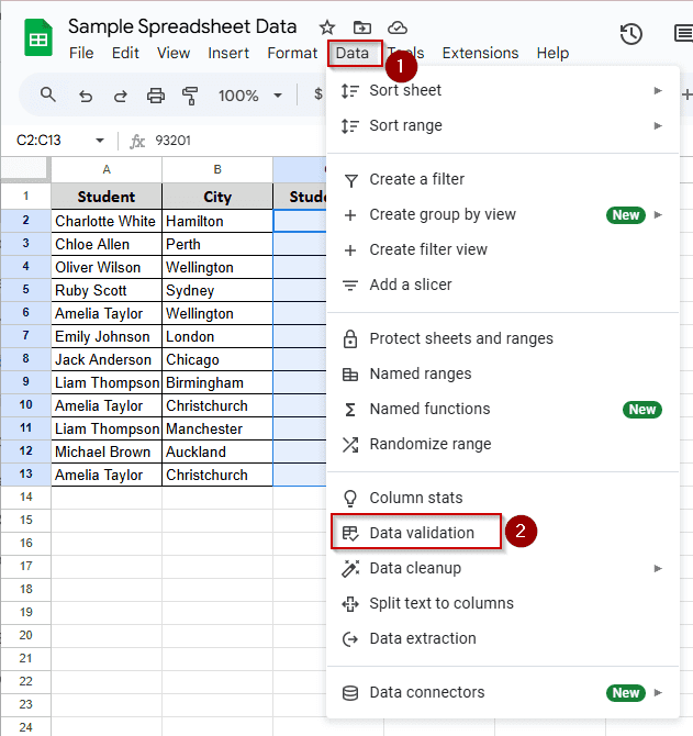
➤ Go to the Data menu at the top and choose Data validation from the drop-down list. You will see the data validation option appear on the right side of your screen.
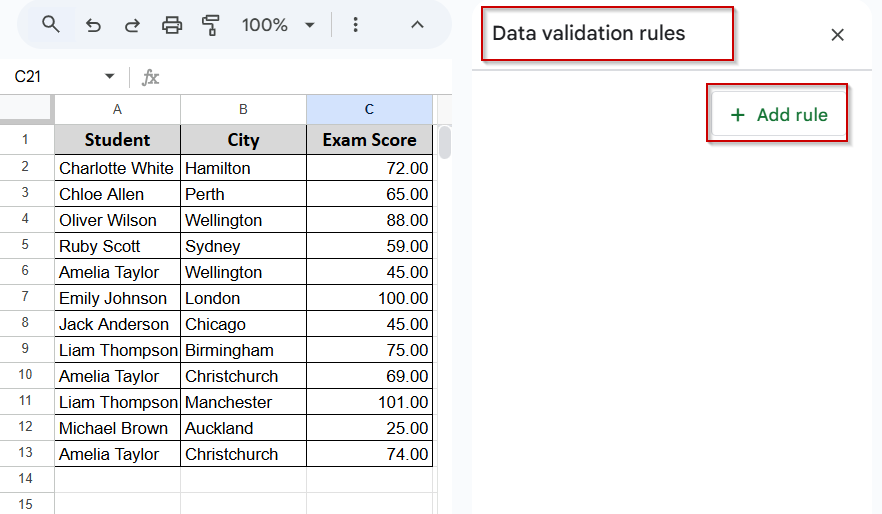
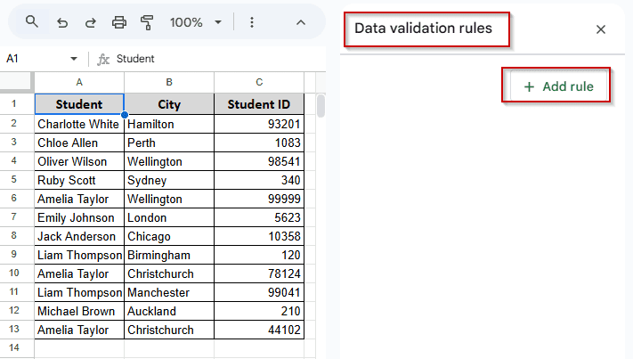
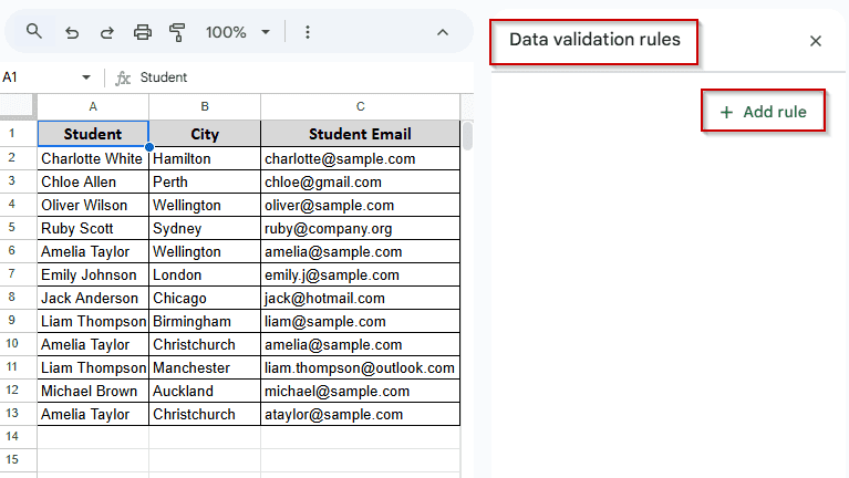
➤ Click on Add Rule. You will see some boxes appear. Don’t get afraid after seeing the bulk of options. Here is what you will do.
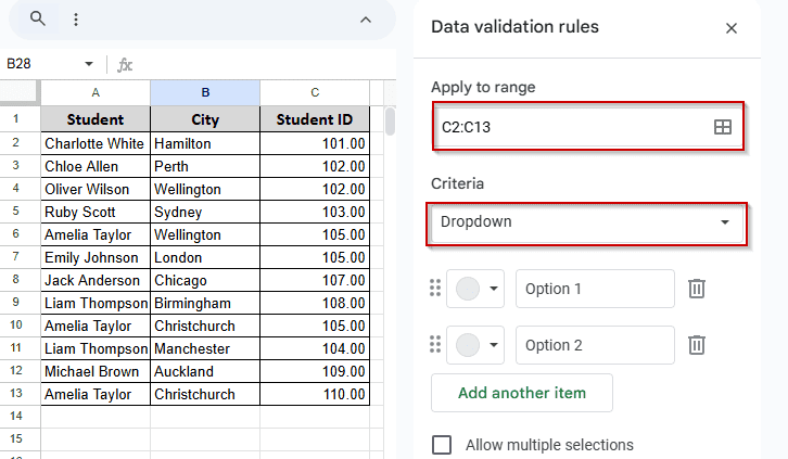
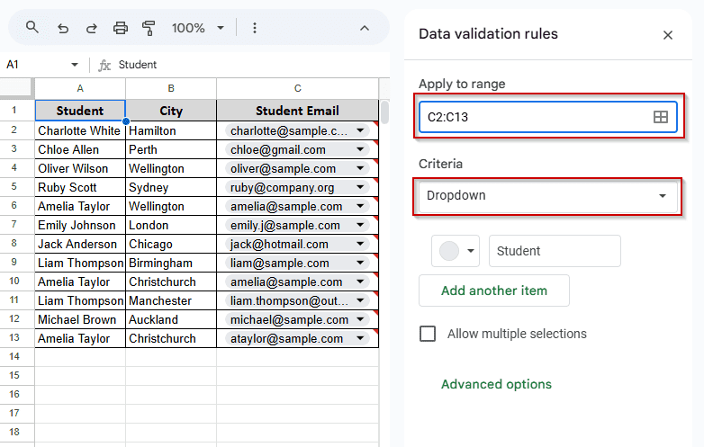
➤ In the Apply to Range box, write down the range only, nothing else. In our case, it is C2:C13.
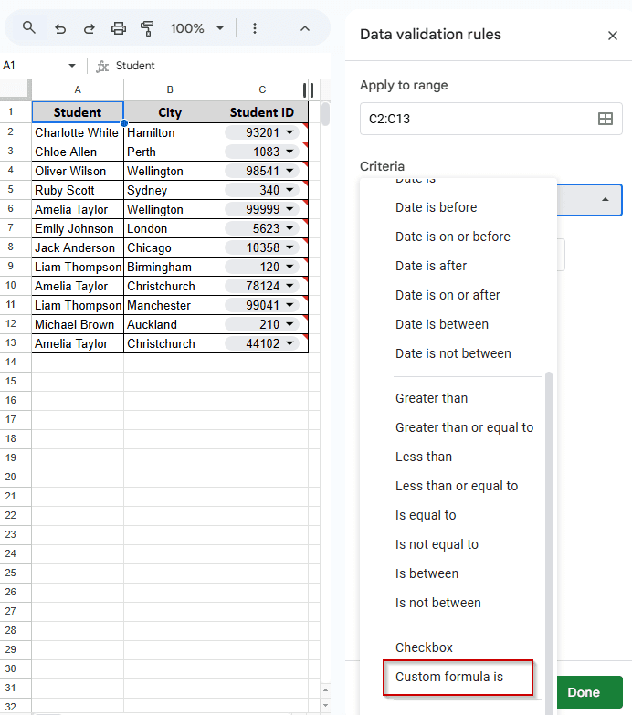
➤ Then, click on the dropdown menu just under where you see Criteria. You should also click on the advanced menu so that we can show a warning sign.
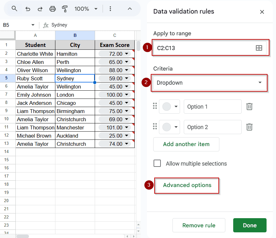
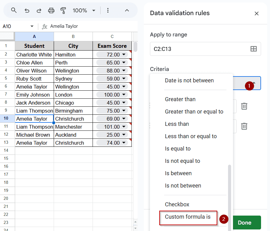
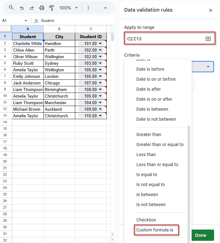
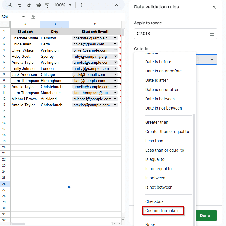
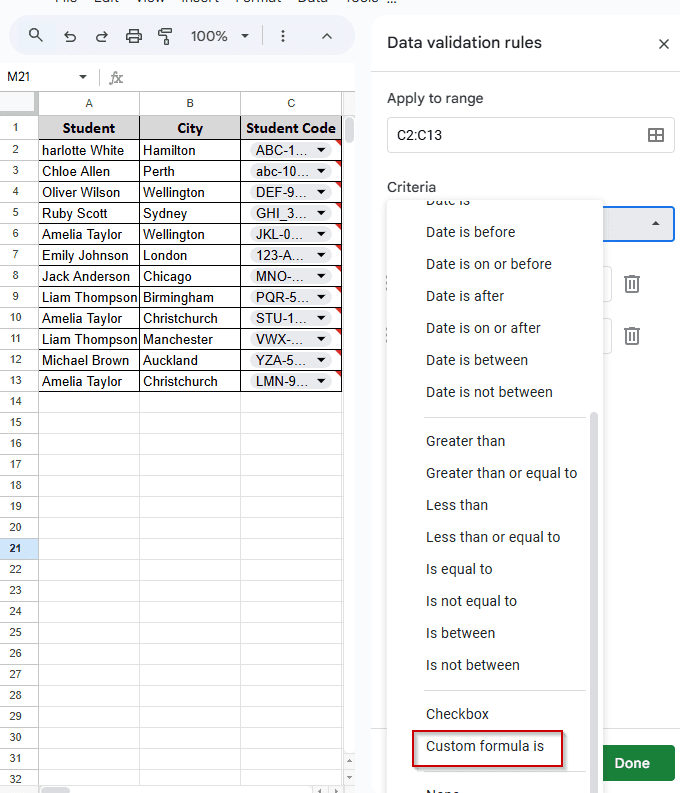
➤ After clicking on the dropdown, you will see a bunch of lists. Scroll down and you will see an option “Custom formula is”. Select this one.
➤ Then, do these one by one. First, insert the formula = AND (ISNUMBER (C2), C2 >= 40, C2=100). This will ensure your data stays within this range. Feel free to change it if you want.
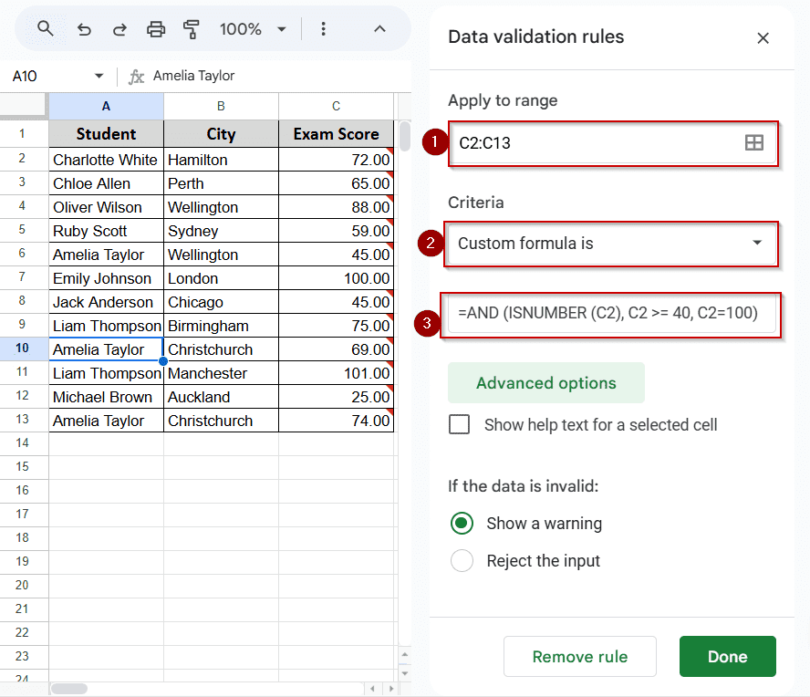
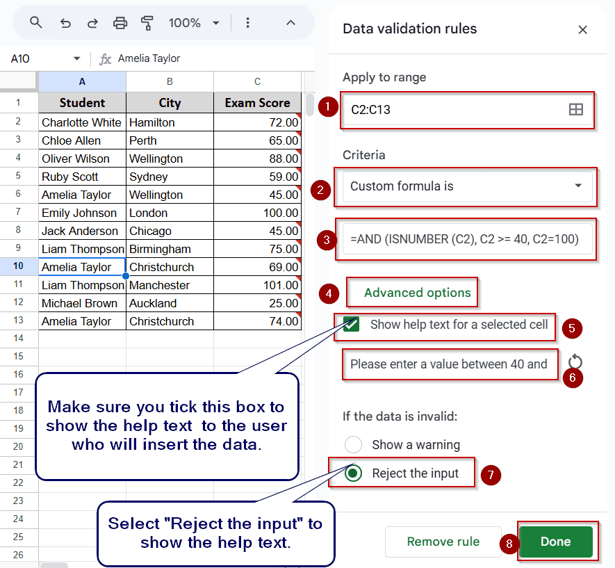
➤ After clicking the Advanced Options, you will see some new options.
➤ Make sure the Show help text for a selected cell is ticked.
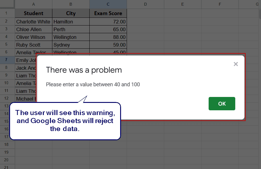
➤ Write your help text in the box below. We wrote, “Please enter a value between 40 and 100.”
➤ Select “Reject Input” from the “If the data is invalid:” option. And click on Done.
Now you will see a red sign at the top right corner of the data that does not meet our validation range. You will see the detailed message after hovering your mouse over the data. In our case, 101 and 25 are not within the range. Therefore, Google Sheets shows a red mark at the top-right corner, and when we hover over it, it displays the detailed message.
➤ Try to insert data that does not meet the range value and you will see the warning sign that you wrote.
That’s it. You have successfully completed the data validation method with a custom formula. Let’s try the next example, where we will find duplicate entries.
Note:
If you don’t select the “Reject input” option, Google Sheets will still accept invalid data and only show a small red mark in the corner. If the user misses it, he or she will continue inserting data that violates the validation. So, always check the Reject input radio button.
Duplicate Entry Validation
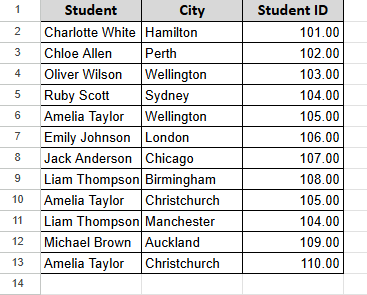
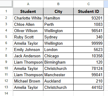
In the following dataset, we have a list of students in Column A and their cities in Column B. In the third column (Column C), we’ve added their Student ID.
Now, what we want is to make sure the values in the Student ID column are unique. That means each student should have a different ID. So, if someone tries to insert the same ID twice, Google Sheets will not accept it.
Let’s begin.
➤ Select the Student ID cells. In this case, from C2 to C13.
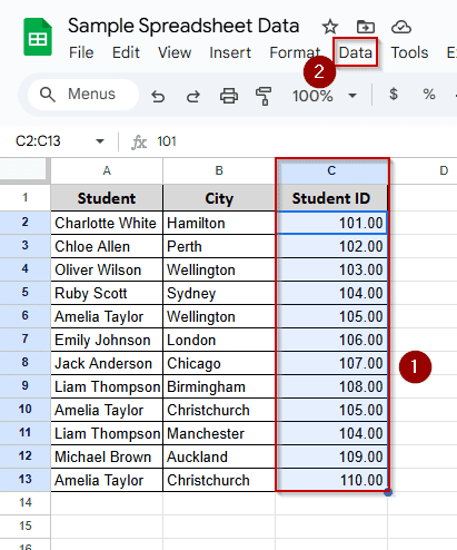
➤ Go to the Data menu at the top and choose Data validation from the drop-down list.

➤ You will see the data validation option appear on the right side of your screen.
➤ Click on Add Rule. You will see some boxes appear, just as you saw in the previous method.
➤ In the Apply to Range box, write down the range only, nothing else. In our case, it is C2:C13.
➤ Then, click on the dropdown menu just under where you see Criteria.
➤ After clicking on the dropdown, you will see a bunch of lists. Scroll down and you will see an option “Custom formula is”. Select this one.
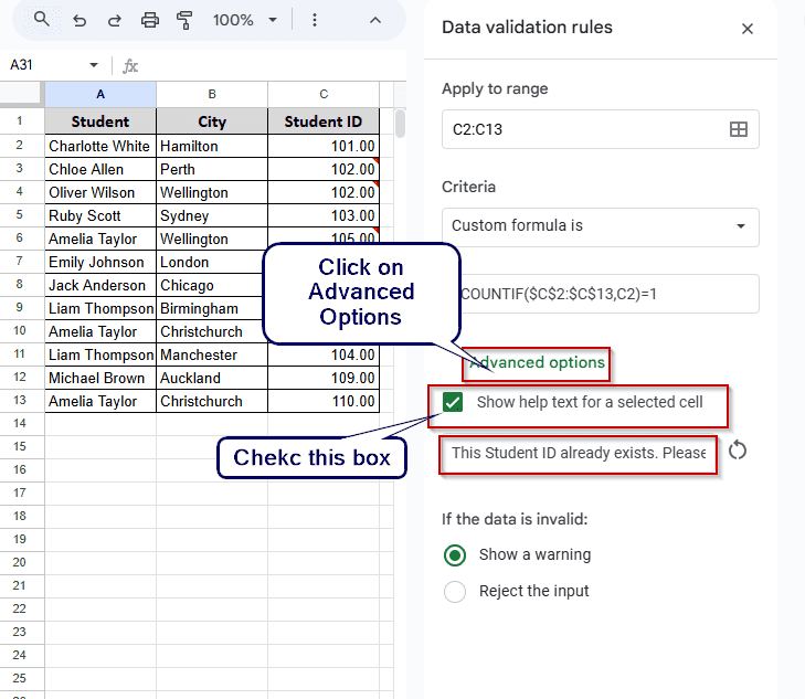
➤ Then, do these one by one. First, insert the formula =COUNTIF($C$2:$C$13,C2)=1. This will ensure that every Student ID entered in Column C appears only once.
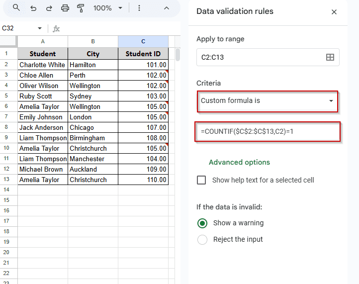
➤ After clicking the Advanced Options, you will see some new options.
➤ Make sure the Show help text for a selected cell is ticked.
➤ Write your help text in the box below. We wrote, “This Student ID already exists. Please enter a unique ID.”
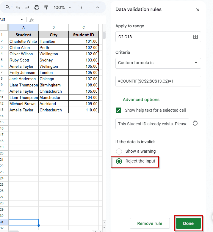
➤ Select “Reject Input” from the “If the data is invalid:” option. And click on Done.
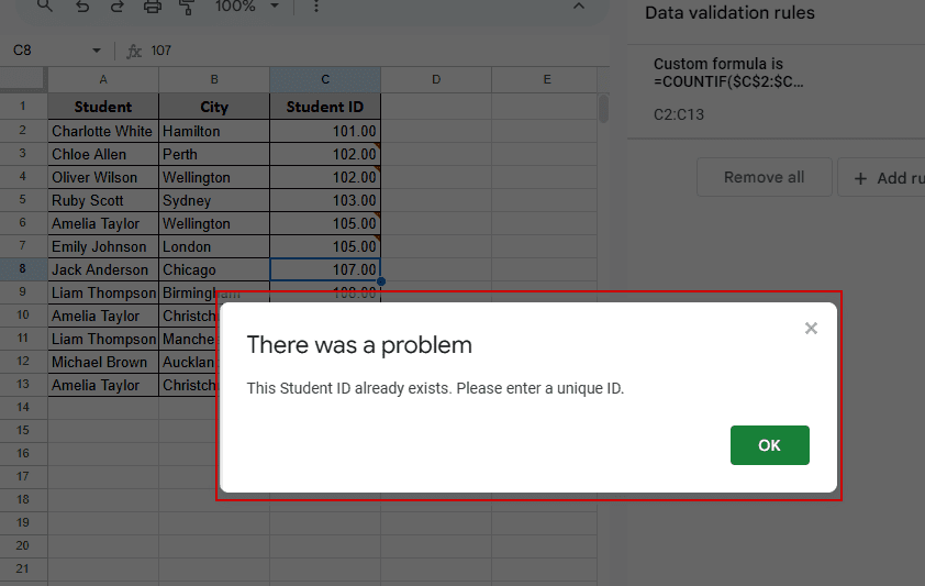
➤ Now try to enter a duplicate Student ID in Column C. If the ID already exists in the list and you will see the error message.
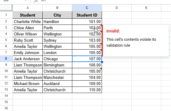
➤ And you will see red marks at the top right corner of all IDs that violate the rule, and now you can remove all the duplicate inputs.
That’s it. You have successfully completed the duplicate entry validation using a custom formula. Let’s go to the next one, where we will check for a length-based validation.
Length-Based Validation
In the following dataset, we have a list of students in Column A and their cities in Column B. In the third column (Column C), we’ve added their Student ID.
What we want is to make sure the Student ID has exactly five digits. No more and no less. If anyone tries to enter an ID with four or six digits, or something with letters, Google Sheets will reject that.
➤ Select the Student ID cells. In this case, from C2 to C13.
➤ Go to the Data menu at the top and choose Data validation from the drop-down list.
➤ You will see the data validation option appear on the right side of your screen. Click on Add Rule.
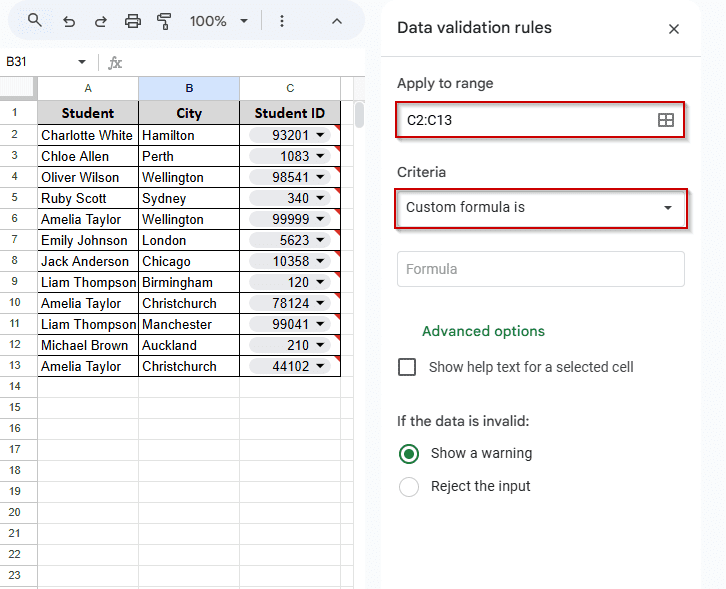
➤ In the Apply to Range box, write down the range only, nothing else. In our case, it is C2:C13.
➤ Then, click on the dropdown menu just under where you see Criteria.

➤ After clicking on the dropdown, you will see a bunch of lists. Scroll down and you will see an option “Custom formula is”. Select this one.
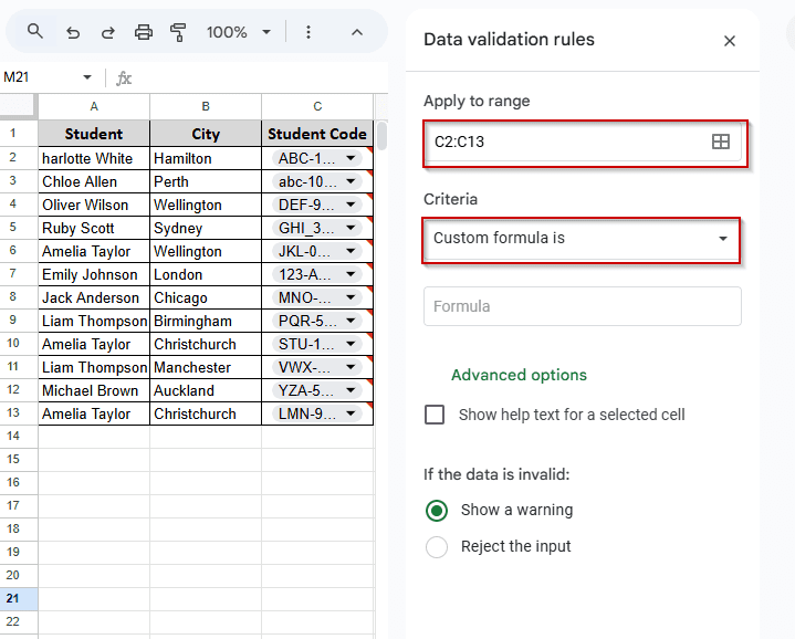
➤ The data validation section will now look like this.
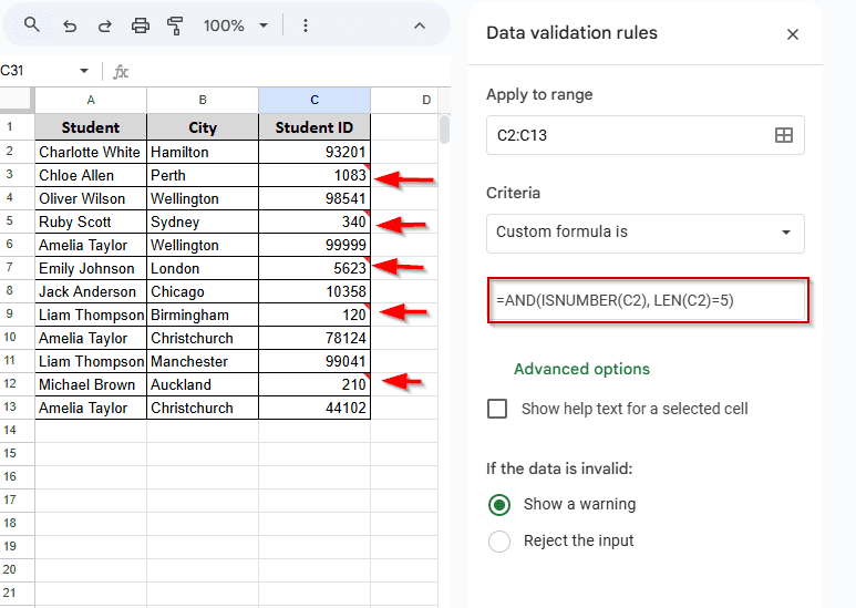
➤ Then, do these one by one. First, insert the formula =AND(ISNUMBER(C2), LEN(C2)=5). This will ensure that the Student ID has exactly five digits. You will immediately see a red mark at the top right corner of those ID numbers that violate the rule.
➤ Now, click on the Advanced Options, and you will see some new options.
➤ Make sure the Show help text for a selected cell is ticked.
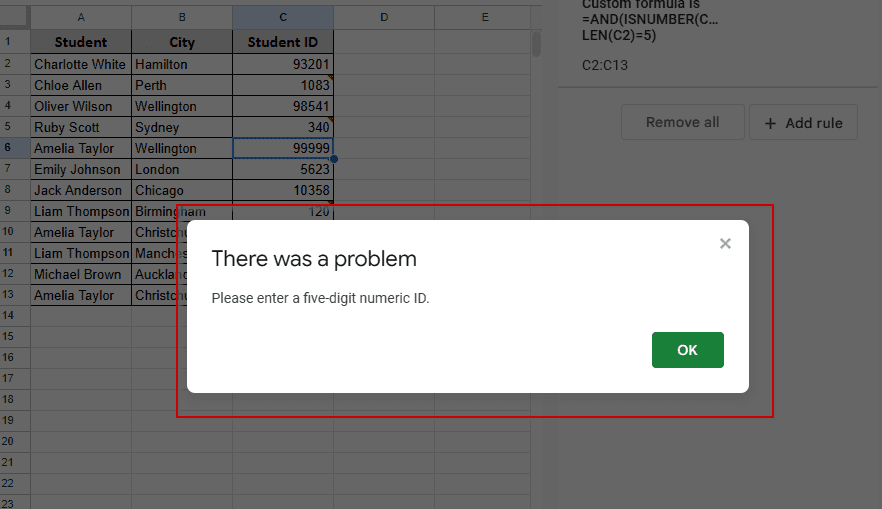
➤ Write your help text in the box below. We wrote, “Please enter a five-digit numeric ID.”
➤ Select “Reject Input” from the “If the data is invalid:” option. And click on Done.

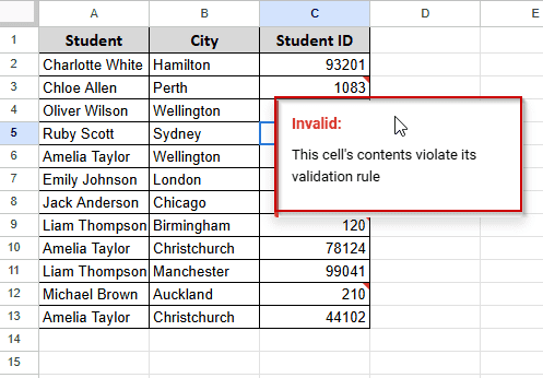
➤You will see a red mark at the top-right corner of the data that is not 5 digits. Hover over your muse, and you will see a more detailed message.
➤ Now try to enter an ID with fewer or more than five digits. Google Sheets will not accept the value, and a pop-up will appear with the warning sign you wrote in the help box.
That’s it. Now let’s learn how to validate email in Google Sheets.
Domain-Specific Email Validation
In the following dataset, we have a list of students in Column A and their cities in Column B. In the third column (Column C), we’ve added their email addresses.
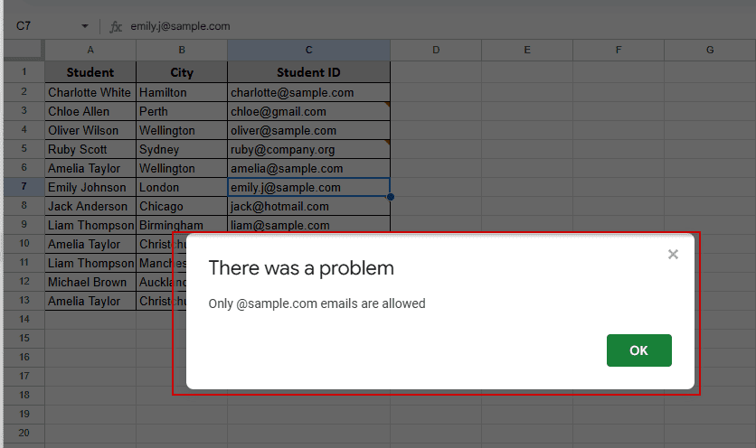
Now, what we want is to make sure all email addresses end with @sample.com. If someone enters Gmail, Yahoo, or anything else, Google Sheets will reject the data.

➤ Select the Email cells. In this case, from C2 to C13.
➤ Go to the Data menu at the top and choose Data validation from the drop-down list.
➤ You will see the data validation option appear on the right side of your screen.
➤ Click on Add Rule. You will see some boxes appear.
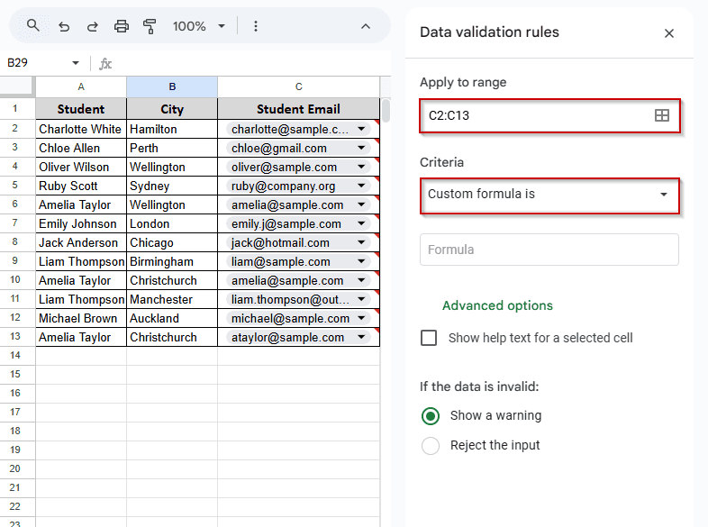
➤ In the Apply to Range box, write down the range only, nothing else. In our case, it is C2:C13.
➤ Then, click on the dropdown menu just under where you see Criteria.
➤ After clicking on the dropdown, you will see a bunch of lists. Scroll down and you will see an option “Custom formula is”. Select this one.
➤ The data validation section will now look like this.
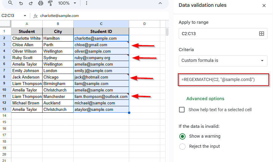
➤ Then, do these one by one. First, insert the formula =REGEXMATCH(C2, “@sample.com$”). This will make sure the email ends with @sample.com. You will immediately see a red mark at the top right corner of those emails that violate the rule.
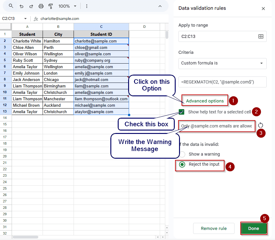
➤ After clicking the Advanced Options, you will see some new options.
➤ Make sure the Show help text for a selected cell is ticked.
➤ Write your help text in the box below. We wrote, “Only @sample.com emails are allowed.”
➤ Select “Reject Input” from the “If the data is invalid:” option. And click on Done.
➤You will see a red mark at the top-right corner of the data that is not following the domain rule. Hover over your mouse, and you will see a more detailed message.
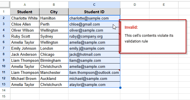
➤ Now, try to enter any email that does not end in @sample.com. You will see the warning message that you entered earlier.
That’s it. You have successfully completed the domain-specific email validation using a custom formula. Let’s go to the next one, where we will check for a specific input pattern using regex.
Pattern-Based Validation with Regex
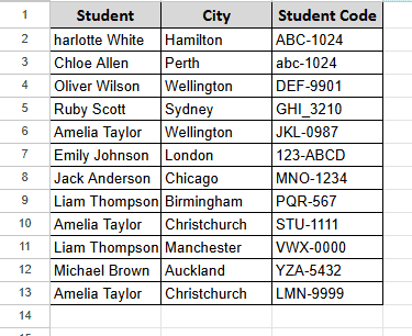
In the following dataset, we have a list of students in Column A and their cities in Column B. In the third column (Column C), we’ve added their Student Code.
Now, what we want is to make sure all the codes follow the same pattern. Each code should be in the format of three uppercase letters, a hyphen, and then four digits. For example: ABC-1234. Any code that does not follow this pattern, Google Sheets will reject those.
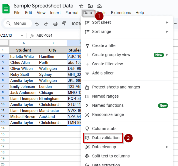
➤ Select the Student Code cells. In this case, from C2 to C13.
➤ Go to the Data menu at the top and choose Data validation from the drop-down list.
➤ You will see the data validation option appear on the right side of your screen.
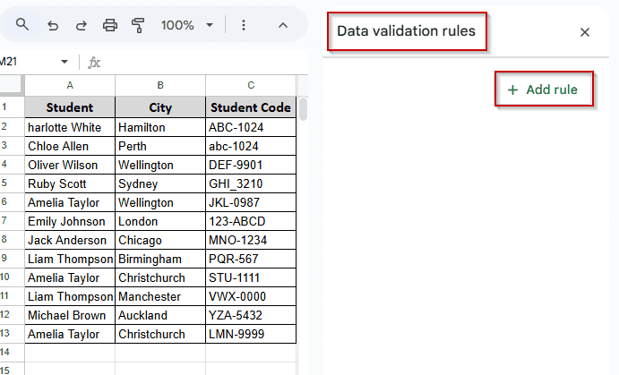
➤ In the Apply to Range box, write down the range only, nothing else. In our case, it is C2:C13.
➤ Then, click on the dropdown menu just under where you see Criteria.
➤ After clicking on the dropdown, you will see a bunch of lists. Scroll down and you will see an option “Custom formula is”. Select this one.
➤ The Data Validation section will look like this now.
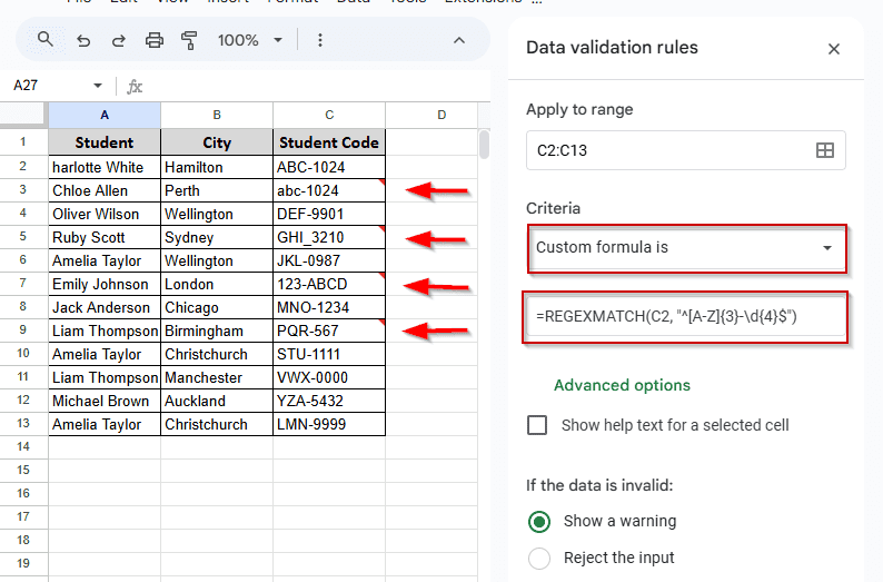
➤ Then, do these one by one. First, insert the formula =REGEXMATCH(C2, “^[A-Z]{3}-\d{4}$”). This will make sure the input follows the exact format: three capital letters, a dash, and four numbers.
➤ You will immediately see a red mark at the top right corner of those codes that violate the rule.
➤ After clicking the Advanced Options, you will see some new options.
➤ Make sure the Show help text for a selected cell is ticked.
➤ Write your help text in the box below. We wrote, “Enter a code in the format ABC-1234.”
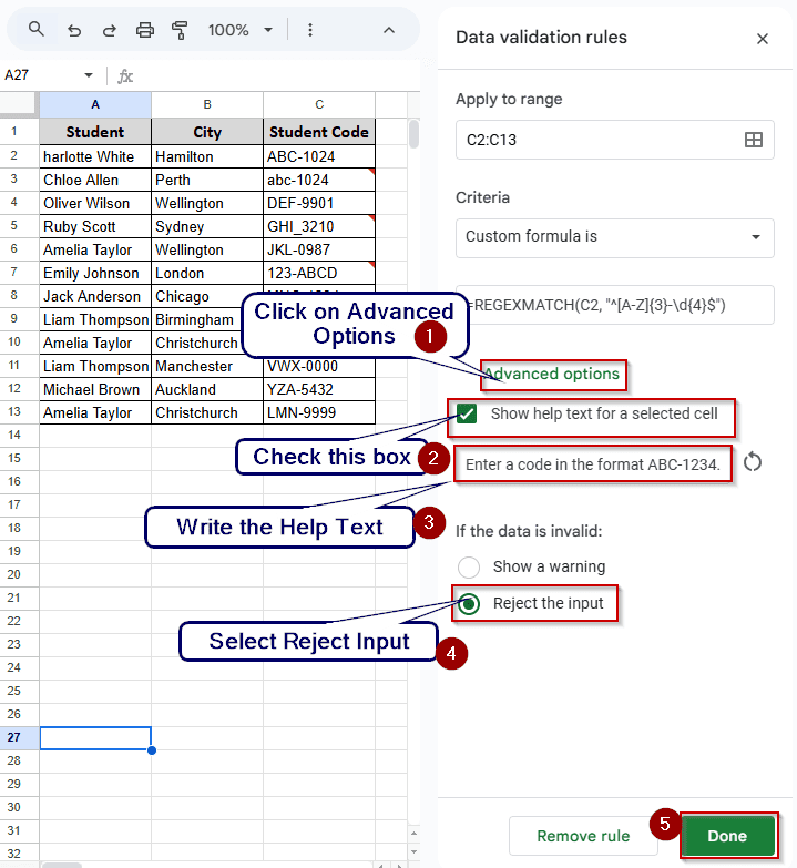
➤You will see a red mark at the top-right corner of the data that is not following the code rule. Hover over your mouse, and you will see a more detailed message.
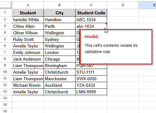
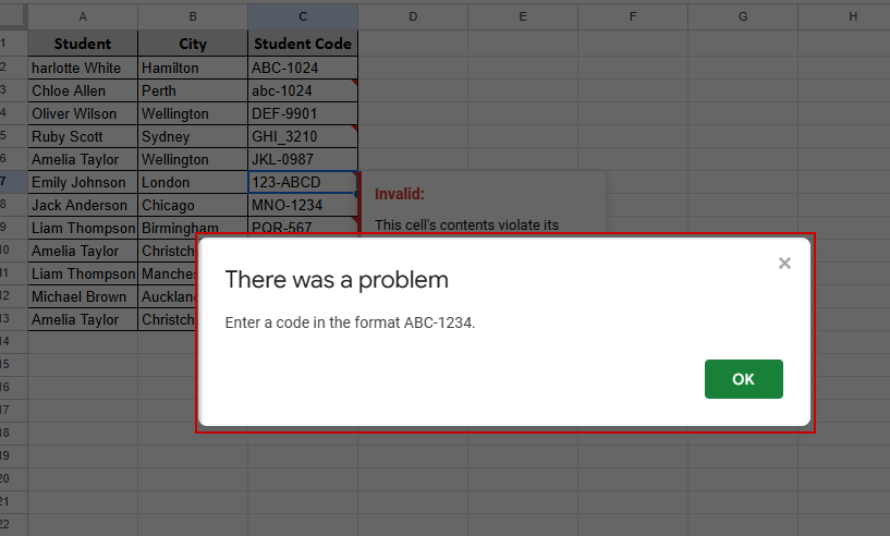
➤ Now try to enter a code like abc-1234, XYZ_0000, or 123-ABCD. Google Sheets will reject the input, and you will see the warning message that you entered earlier.
That’s it. You have successfully completed the pattern-based validation using a custom formula
Frequently Asked Questions
What types of functions are supported in custom formula validation?
You can use any function that returns TRUE or FALSE. You can use Functions like ISNUMBER, LEN, COUNTIF, REGEXMATCH, AND, and OR. If your formula doesn’t return TRUE or FALSE, the validation won’t work.
Can I use FILTER or VLOOKUP directly in custom formula validation?
No, you can’t use those functions directly in the data validation formula box. Google Sheets does not support that. If you really need them, you can use a helper column instead.
Why does Google Sheets reject my custom formula rule without error?
This usually happens when your formula doesn’t match your selected range. For example, if you start from C2, your formula should also refer to C2, not any other cell. You should also make sure your formula returns True or False.
Is there a limit to how many rows a custom formula validation can cover?
No. There is no official limit. But if you apply a custom formula to a huge range (let’s say over thousands), then it can make the process slow; in the worst case, the browser can be non-responsive.
Can I use REGEXMATCH in both data validation and conditional formatting?
Yes, you can and you should do that. It works better for checking emails, codes, or a specific keyword.
Concluding Words
In this article, you learned how to apply data validation in Google Sheets using custom formulas. We have shown you 5 different methods and examples. We showed with use cases so you can learn where you should use a custom formula.
We have added the worksheet. You can download the worksheet for practice purposes. Also, if you have any specific problems or questions, please ask us in the comment box below.