Looking up values from left to right using VLOOKUP is a common task in Google Sheets. But what if your lookup value is on the right and you need to return a matching value from the left? VLOOKUP won’t work in that case, but don’t worry, there are easy alternatives.
In this article, you’ll learn multiple ways to perform a reverse VLOOKUP in Google Sheets using functions like INDEX, MATCH, ARRAYFORMULA, QUERY, and FILTER. These methods help you retrieve data from the left of your lookup value, giving you more flexibility when working with real-world datasets.
Steps to perform a basic reverse lookup in Google Sheets using the VLOOKUP function with an array literal:
➤ Use the dataset in cells A1:C11, with columns for Product ID, Category, and Product Name.
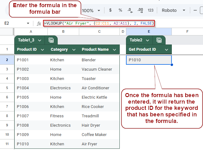
➤ To retrieve the Product ID for a given Product Name (e.g., “Air Fryer”), enter this formula in cell E2:
=VLOOKUP(“Air Fryer”, {C2:C11, A2:A11}, 2, FALSE)
➤ Press Enter to return P1010, the Product ID for “Air Fryer”.
Basic REVERSE Lookup in Google Sheets
If you want to pull values from a column to the left of your search column, something the standard VLOOKUP function doesn’t support on its own, a reverse lookup becomes necessary. The simplest way to do this is by combining VLOOKUP with an array literal. This method lets you flip the column order inside the formula so you can retrieve left-side data based on a right-side match.
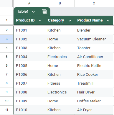
This is the dataset we will be using to demonstrate the methods:
Steps:
➤ Use the dataset in cells A1:C11, where columns represent Product ID, Category, and Product Name, from left to right.
➤ To perform a reverse lookup that returns the Product ID based on the Product Name, enter the following formula in cell E2:
=VLOOKUP(“Air Fryer”, {C2:C11, A2:A11}, 2, FALSE)
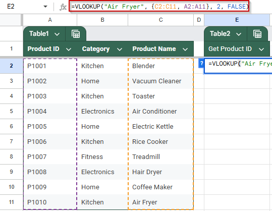
➧ {C2:C11, A2:A11}: Combines Product Name and Product ID into a virtual table with Product Name on the left.
➧ 2: Tells VLOOKUP to return the second column from this virtual table, which is the Product ID.
➧ FALSE: Ensures an exact match is returned.
➤ Press Enter, and the formula will return P1010, which is the Product ID for “Air Fryer”.
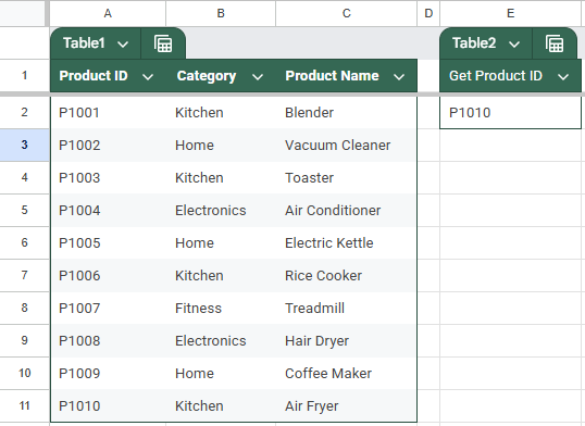
➤ This is the most straightforward way to perform a reverse lookup using VLOOKUP in Google Sheets when your return column is to the left of the lookup column.
Perform a Reverse VLOOKUP Using INDEX and MATCH in Google Sheets
Standard VLOOKUP functions in Google Sheets only allow you to search for a value in the first column of a range and return a value to the right. However, sometimes you need to look up a value from a column to the right and return a related value from a column to the left. The combination of INDEX and MATCH functions offers a flexible and powerful way to perform this “reverse lookup.” This method searches for a specific value in one column and returns a corresponding value from any other column in the dataset, regardless of their order.
Steps:
➤ Use the dataset in cells A1:C11, where columns represent Product ID, Category, and Product Name, from left to right.
➤ To look up the Product ID for a given Product Name using INDEX and MATCH, enter the following formula in cell F3:
=INDEX(A2:A11, MATCH(F2, C2:C11, 0))
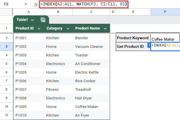
(Assume F2 contains the product name you want to search for, e.g., “Coffee Maker”)
➧ INDEX(A2:A11, ...): Retrieves the value from the Product ID column at the same row as the matched product name.
➧ 0: Ensures an exact match.
➤ Press Enter, and the formula will return P1009, which is the Product ID for “Coffee Maker”.
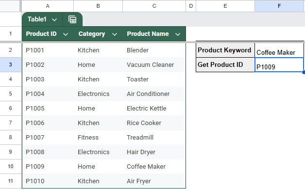
➤ This method gives you a dynamic, left-direction lookup and works even if your columns are rearranged, unlike standard VLOOKUP.
Apply ArrayFormula for Enhanced Reverse Lookups in Google Sheets
When you need to perform multiple reverse lookups at once, using the combination of INDEX and MATCH inside an ARRAYFORMULA can save time and make your spreadsheet more dynamic. This method allows you to look up several product names in a column and return their corresponding Product IDs all at once, without needing to copy the formula row by row. It’s especially helpful for handling large datasets or automating repetitive lookups.
Steps:
➤ Use the dataset in cells A1:C11, where columns represent Product ID, Category, and Product Name.
➤ Suppose you have a list of product names in column E (E2:E5), and you want to return their Product IDs in column F. Enter the following formula in F2:
=ARRAYFORMULA(IF(E2:E5=””, “”, IFERROR(VLOOKUP(E2:E5, {C2:C11, A2:A11}, 2, FALSE), “Not Found”)))
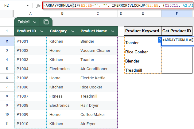
➧ {C2:C11, A2:A11}: This creates a temporary table with Product Names in the first column and Product IDs in the second, allowing a right-to-left lookup.
➧ VLOOKUP(E2:E5, ..., 2, FALSE): Searches for each Product Name in the first column of the virtual table and returns the corresponding Product ID from the second column.
➧ IFERROR(..., "Not Found"): If a Product Name isn’t found, this avoids showing an error and instead displays "Not Found."
➧ ARRAYFORMULA(...): Enables the formula to work over a range (E2:E5), returning results row-by-row without needing to drag the formula down manually.
➧ IF(E2:E5="", "", ...): Ensures that if a cell in E2:E5 is blank, the output will also be blank rather than "Not Found" or an error.
➤ Press Enter, and the formula will output the matching Product IDs for all product names in column E, dynamically updating as you add or change product names.
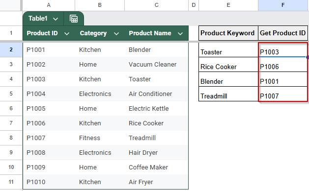
➤ This method is ideal for bulk reverse lookups, enhancing efficiency and minimizing manual work.
Utilize QUERY for Advanced Reverse Lookups in Google Sheets
The QUERY function is a powerful tool that can perform complex data retrievals similar to database queries. Using QUERY for reverse lookups allows you to find a Product ID by searching for a Product Name with great flexibility. This method is especially useful if you want to filter, sort, or apply conditions while doing your reverse lookup, all within a single formula.
Steps:
➤ Use the dataset in cells A1:C11, where columns represent Product ID, Category, and Product Name.
➤ Suppose you want to look up the Product ID for the product name entered in cell F1. Enter the following formula in cell F2:
=QUERY(A2:C11, “SELECT A WHERE C = ‘” & F2 & “‘”, 0)
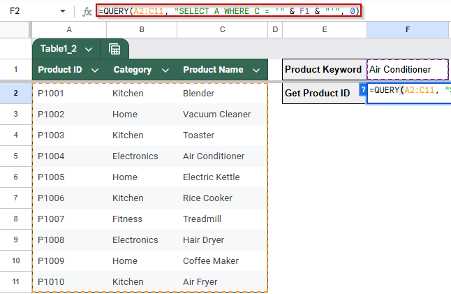
➧ The QUERY statement that selects Product IDs (A) where the Product Name (C) matches the value in cell F1.
➧ The 0 at the end indicates that the dataset has headers in the first row.
➤ Press Enter, and the formula will return the Product ID matching the product name in F1.
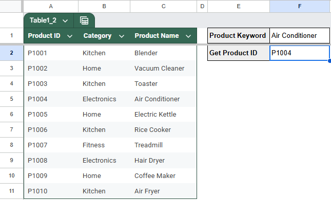
➤ This method is ideal when you want to apply more complex conditions or need a dynamic reverse lookup with the power of Google Sheets’ query language.
Use FILTER for Dynamic Reverse Lookups in Google Sheets
The FILTER function offers a powerful and flexible way to perform reverse lookups by returning all matching values based on a specified condition. It is especially useful when you expect multiple matches or want your results to update automatically as your data changes. This method is ideal for dynamic datasets where product names might appear more than once.
Steps:
➤ Use the dataset in cells A1:C11, where columns represent Product ID, Category, and Product Name.
➤ To retrieve the Product ID for a product name entered in cell F1, input this formula in cell F2:
=FILTER(A2:A11, C2:C11 = F1)
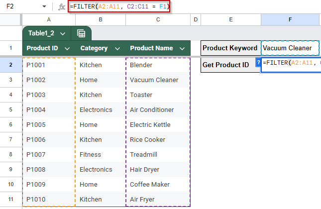
➧ C2:C11 = F1: Filters Product IDs where the Product Name matches the value in F1.
➤ Press Enter to display the Product ID(s) corresponding to the product name entered.
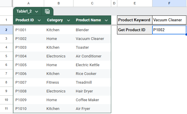
➤ This method dynamically updates results and can handle multiple matches efficiently.
Frequently Asked Questions
What is a reverse VLOOKUP in Google Sheets?
A reverse VLOOKUP searches for a value in the last column of a table and returns the corresponding value from an earlier column. It’s useful when the lookup value isn’t in the first column, unlike traditional VLOOKUP.
Why use INDEX and MATCH instead of VLOOKUP for reverse lookups?
INDEX and MATCH offer flexibility to look up values in any column, regardless of position. Unlike VLOOKUP, they don’t require the lookup value to be in the first column, making them ideal for reverse lookups or complex table arrangements.
Can I use ArrayFormula with reverse lookup formulas?
Yes, ArrayFormula allows you to apply reverse lookup formulas to entire ranges dynamically. This is helpful for large datasets or when you want your lookup to automatically adjust without manually copying formulas row by row.
How does the QUERY function help in reverse lookups?
QUERY can perform SQL-like searches on your dataset, filtering and returning rows based on conditions. It’s powerful for complex reverse lookups where you need to combine filtering, sorting, or multiple conditions in a single formula.
What are the advantages of using FILTER for reverse lookups?
FILTER returns all matching results dynamically and updates automatically when data changes. It’s excellent for reverse lookups that may have multiple matches, allowing you to see every relevant result instead of just the first one.
Wrapping Up
Reverse VLOOKUPs in Google Sheets may seem tricky at first, especially since the standard VLOOKUP function doesn’t support looking to the left. But with the right tools, like INDEX and MATCH, ARRAYFORMULA, QUERY, and FILTER, you can perform powerful and flexible reverse lookups that adapt to your data structure. Whether you need a simple one-time lookup or a dynamic solution that scales across your sheet, the methods in this article will help you pull values from the left side of a dataset quickly and accurately.