The VLOOKUP function in Google Sheets is powerful, but it can sometimes return a frustrating error: “Did not find value in VLOOKUP evaluation.” This message usually means Google Sheets couldn’t locate the value you’re searching for, often due to small issues in formatting, lookup structure, or incorrect parameters.
In this article, we’ll walk you through the most common reasons why this error occurs and show you practical ways to fix it. Whether it’s extra spaces, incorrect ranges, or data type mismatches, each solution comes with examples so you can troubleshoot with confidence.
Steps to avoid the “Did not find value in VLOOKUP evaluation” error in Google Sheets by structuring the formula correctly:
➤ Use the dataset in cells A1:C11, with columns for Product ID, Product Name, and Price.
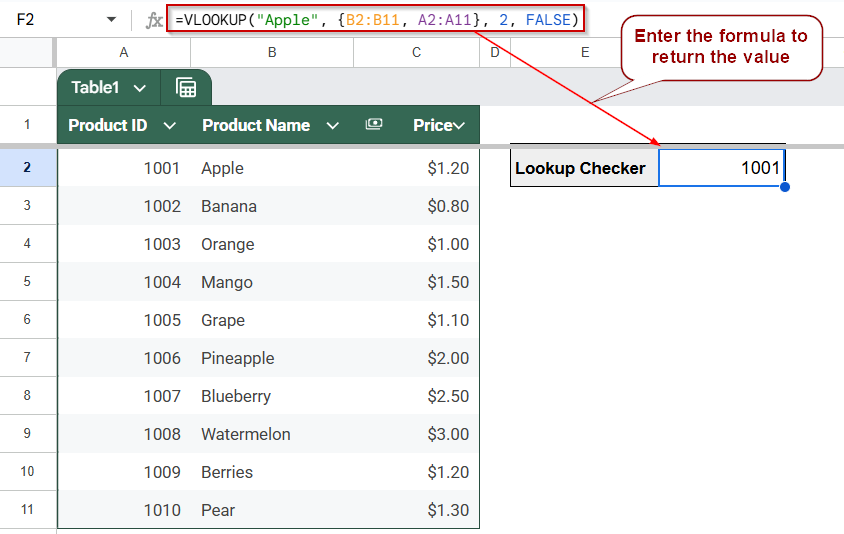
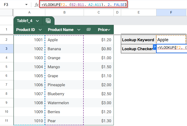
➤ To retrieve the Product ID based on a Product Name (e.g., “Apple”), enter this formula in cell F2:
=VLOOKUP(“Apple”, {B2:B11, A2:A11}, 2, FALSE)
➤ Make sure the lookup column (Product Name) is first in the array.
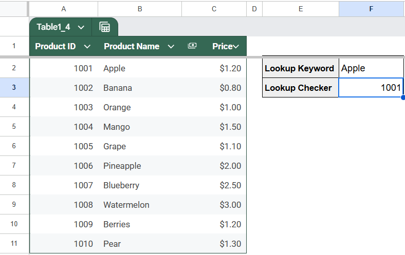
➤ Press Enter to return 1001, the Product ID for “Apple”.
Check for Exact Match Lookup Errors in VLOOKUP
One of the most frequent causes of the “Did not find value in VLOOKUP evaluation” error is a mismatch between the lookup value and the data in your table. When you use the FALSE argument in VLOOKUP, it demands an exact match. Even a small typo or an extra space can break it. This method helps you trace and fix such issues.
Steps:
➤ Use the dataset in cells A1:C11, where columns represent Product ID, Product Name, and Price.
➤ Add lookup values in cells F2, such as “Grapefruit” (intentionally not in the dataset), etc.
➤ To retrieve the Product ID based on a product name, enter this formula in cell F3:
=VLOOKUP(F2, {B2:B11, A2:A11}, 2, FALSE)
➤ You’ll see #N/A if the value in D2 is misspelled or not found in the Product Name list. In our case, the dataset does not contain any keyword called “Grapefruit”
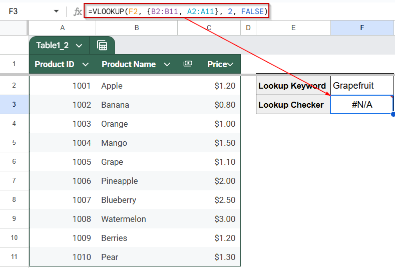
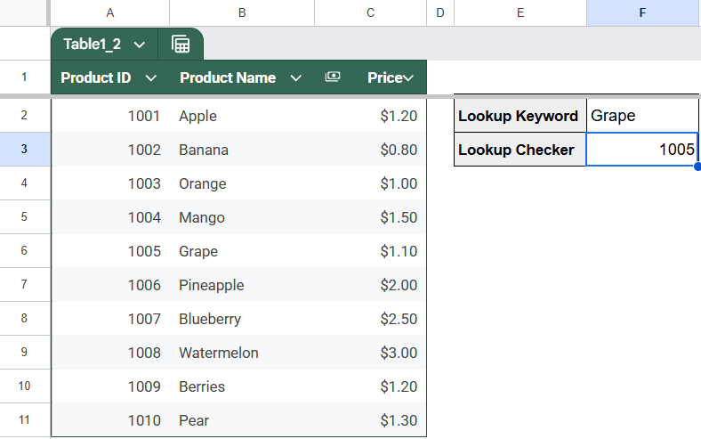
➤ The dataset contains the keyword “Grape”. Fix the keyword, and the formula should work now.
➤ Always double-check that your lookup keyword is clean and appears exactly in the target range.
Remove Extra Spaces Using the TRIM Function
When VLOOKUP returns an #N/A error, the problem may not be a missing value, but hidden spaces. Extra spaces at the beginning, end, or within text can prevent exact matches even when the values look identical. This method uses the TRIM function to clean both the lookup value and the dataset for reliable reverse lookups.
Steps:
➤ Use the dataset in cells A1:C11, with columns for Product ID, Product Name, and Price.
➤ Enter your lookup keyword (e.g., “Apple”, possibly with hidden spaces) in cell F2.
➤ In cell F3, use the following formula to return the Product ID:
=VLOOKUP(TRIM(F2), ARRAYFORMULA({TRIM(B2:B11), A2:A11}), 2, FALSE)
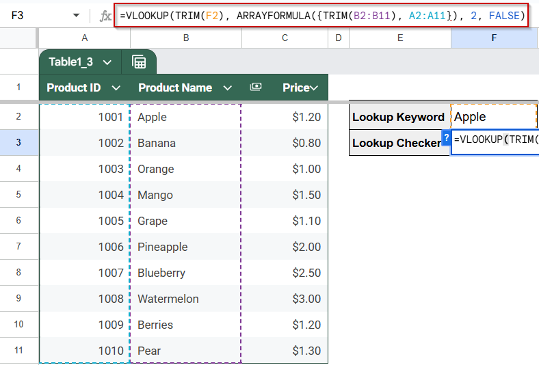
➧ ARRAYFORMULA({TRIM(B2:B11), A2:A11}): Applies TRIM to each entry in the Product Name column and pairs it with the Product ID column.
➧ 2: Tells VLOOKUP to return the second column from this temporary array, which is Product ID.
➧ FALSE: Forces VLOOKUP to find an exact (cleaned) match only.
➤ Press Enter. It should now return the Product ID.

➤ This formula is useful if your data was copy-pasted or imported from external sources, where formatting issues are common.
➤ Hidden spaces are nearly invisible but can silently break lookup operations.
➤ Always consider cleaning your data with TRIM if lookups behave unpredictably.
Correct Data Type Mismatches with VALUE or TO_TEXT
VLOOKUP errors can also happen when the lookup value and the data you’re searching in are of different data types. For example, if your lookup value is a number stored as text, but your table contains actual numbers, VLOOKUP won’t recognize a match, even if the values look the same. This method helps you align data types to ensure a successful lookup.
Steps:
➤ Use the dataset in cells A1:C11, where columns represent Product ID, Product Name, and Price.
➤ If your lookup value is stored as text but the Product IDs in the table are numbers, use this formula in cell F3:
=VLOOKUP(F2, {B2:B11, A2:A11}, 2, FALSE)
➤ Press Enter.
➤ Alternatively, if your table has Product IDs stored as text and your lookup value is numeric, use:
=VLOOKUP(F2, A2:C11, 2, FALSE)
➤ Press Enter to get the correct Product Name.
➤ This method is useful when importing data from external sources where formatting issues are common.
Fix Column Index Number Errors in VLOOKUP
One of the most common causes of the #N/A error in VLOOKUP is using an incorrect column index number. This happens when you reference a column number that doesn’t exist within the specified range, or if the number points to a column that returns unintended results.
Steps:
➤ Use the dataset in cells A1:C11, where columns represent Product ID, Product Name, and Price.
➤ Suppose you want to retrieve the Product Name using Product ID as the lookup value in cell F2.
➤ You mistakenly enter a formula like this in cell F3:
=VLOOKUP(F2, A2:C11, 4, FALSE)
➤ This returns a #REF! error because column index 4 does not exist in range A2:C11, which only has 3 columns.

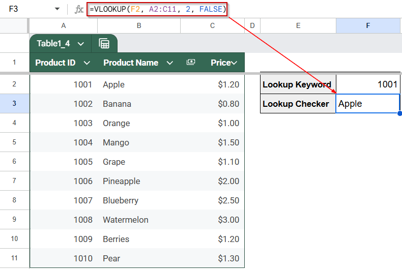
➤ Fix the formula by using the correct index number for the Product Name column, which is 2:
=VLOOKUP(F2, A2:C11, 2, FALSE)
➧ A2:C11: The range where Product ID, Name, and Price are listed.
➧ 2: Tells VLOOKUP to return the second column, Product Name.
➧ FALSE: Ensures the lookup matches the Product ID exactly.
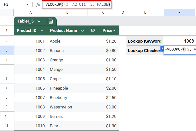
➤ Press Enter, and the formula will return “Watermelon” if F2 contains 1008.
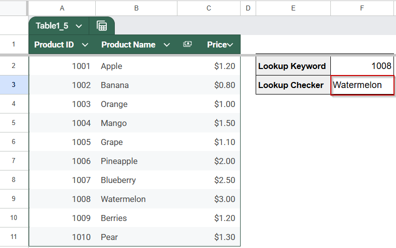
➤ Always check that your column index number is valid for the range and matches the column you actually want to return. To be on the safer side, specify a column index number that is less than the total number of columns you have in your dataset.
Ensure the Lookup Value Is in the First Column of the Range
VLOOKUP requires the lookup value to be in the first column of the defined range. If your lookup column is placed to the right, the formula will not work and will return a #N/A error, even if the value clearly exists in your data.
Steps:
➤ Use the dataset in cells A1:C11, where the columns represent Product ID, Product Name, and Price.
➤ Suppose you want to find the Product ID by looking up the Product Name “Apple”.
➤ If you try this formula in cell F2:
=VLOOKUP(“Apple”, A2:C11, 1, FALSE)
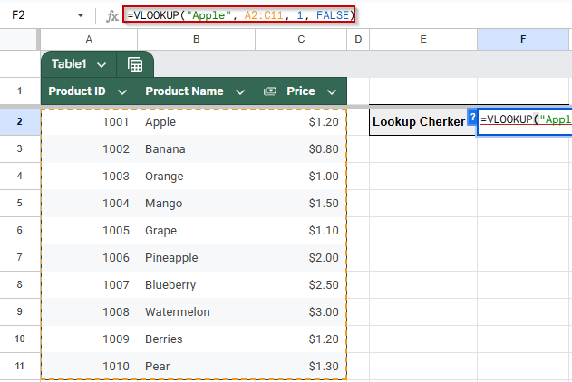
➤ It will return #N/A because column A (Product ID) is the first column, but your lookup value (“Apple”) is in column B (Product Name).

➤ To fix this, rearrange the columns using an array literal so the lookup column comes first:
=VLOOKUP(“Apple”, {B2:B11, A2:A11}, 2, FALSE)
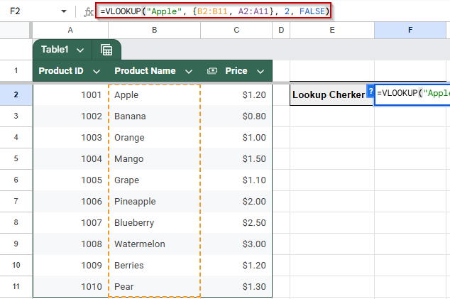
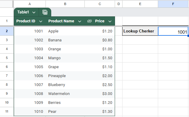
➤ Press Enter, and the formula will return 1001, the Product ID for “Apple”.
➤ Use this method when your lookup column is not the leftmost in your original dataset.
Frequently Asked Questions
Why does VLOOKUP return #N/A even when the value is clearly in the list?
This often happens when there are extra spaces, incorrect capitalization, or data type mismatches in the lookup value or range. VLOOKUP requires an exact match when the fourth argument is set to FALSE.
Can VLOOKUP be used if the lookup column is not the first in the range?
Not directly. VLOOKUP only searches in the first column of the range. You can work around this using an array like {B2:B11, A2:A11} to reorder the columns in the formula.
How do I fix VLOOKUP when it won’t find values with hidden spaces?
Use the TRIM function on both the lookup value and the lookup column to remove hidden spaces. This is especially useful when dealing with imported or copied data.
What happens if I use the wrong column index number in VLOOKUP?
If you reference a column index that’s larger than the number of columns in your range, VLOOKUP returns a #REF! error. Always ensure the index is within the range’s width.
Wrapping Up
The “Did not find value in VLOOKUP evaluation” error in Google Sheets typically happens due to issues like extra spaces, wrong data types, incorrect column index numbers, or the lookup value not being in the first column of the range. Thankfully, each of these problems has a simple fix. By cleaning your data, using functions like TRIM, and ensuring your formula is set up correctly, you can avoid frustrating errors and ensure your lookups return the right results every time.