Ranking in Excel isn’t always about sorting by a single column. Often, you need to break ties or prioritize entries based on multiple rules. Whether you’re ranking within groups, combining multiple conditions, or enforcing a strict hierarchy, Excel has several formula-based methods to handle it.
In this guide, you’ll learn several practical ways to perform multi-criteria ranking using functions like RANK, COUNTIFS, and SUMPRODUCT. Each method is designed for a specific scenario, some create unique ranks, others sort within categories, and a few allow custom ranking logic without helper columns. Let’s get started.
Steps to do ranking in excel based on multiple criteria:
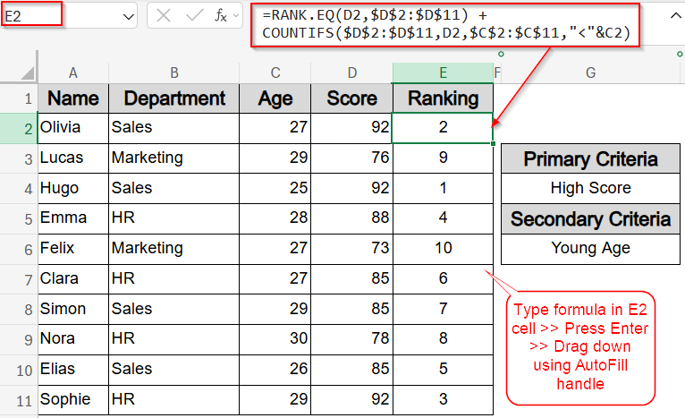
➤ Click cell E2 to begin entering the rank formula.
➤ Type the formula below to rank based on Score and break ties using Age:
=RANK.EQ(D2,$D$2:$D$11) + COUNTIFS($D$2:$D$11,D2,$C$2:$C$11,”<“&C2)
Here, the RANK.EQ function gives the base rank by Score. The COUNTIFS function adds a tie-breaker based on how many rows have the same Score but a smaller Age.
➤ Press Enter.
➤ Drag the fill handle down from E2 to E11 to apply the formula to all rows.
Rank Using Primary and Secondary Criteria with RANK and COUNTIFS Functions
This method ranks each row based on a primary field (like Score) and breaks ties using a secondary field (like age). It’s ideal when you want to assign a clear, unique rank by combining two levels of logic. For example, if two people have the same Score, the younger one will be ranked higher. The final output gives unique ranks that prioritize high performers and resolve ties cleanly using secondary data.
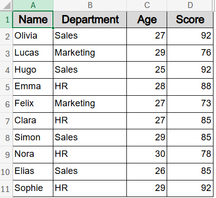
We’ll apply this method to our dataset, where each row includes Name, Department, Age, and Score. The formula will use Score for initial ranking and Age to break ties.
Steps:
➤ Click cell E2 to begin entering the rank formula.
➤ Type the formula below to rank based on Score and break ties using Age:
=RANK.EQ(D2,$D$2:$D$11) + COUNTIFS($D$2:$D$11,D2,$C$2:$C$11,”<“&C2)
Here, the RANK.EQ function gives the base rank by Score. The COUNTIFS function adds a tie-breaker based on how many rows have the same Score but a smaller Age.
➤ Press Enter.
➤ Drag the fill handle down from E2 to E11 to apply the formula to all rows.
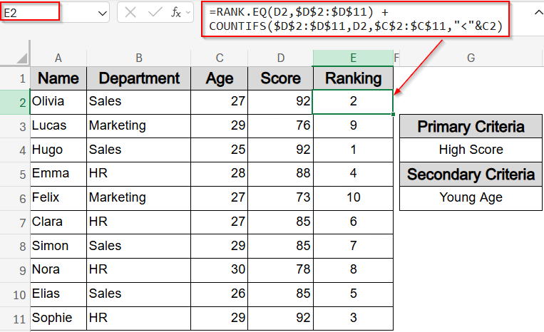
This ranks each row that respects both Score and Age hierarchy.
Assign Unique Ranks Without Duplicates Using COUNTIF and COUNTIFS Functions
This method creates a completely unique ranking by counting how many entries have higher primary values (like Score), then breaks ties by checking how many tied entries have a lower secondary value (like Age). This ensures no duplicate ranks appear in the results, which is ideal for precise ordered lists with multiple criteria.
Steps:
➤ Select cell E2 to enter the rank formula.
➤ Type the following formula to count higher Scores and break ties by Age:
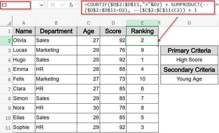
=COUNTIF($D$2:$D$11,”>”&D2) + COUNTIFS($D$2:$D$11,D2,$C$2:$C$11,”<“&C2) + 1
This counts how many scores are greater than the current row’s Score and adds how many tied Scores have a smaller Age. The “+1” adjusts the count into a rank.
➤ Press Enter.
➤ Drag the fill handle down from E2 to E11 to apply the formula to the full range.
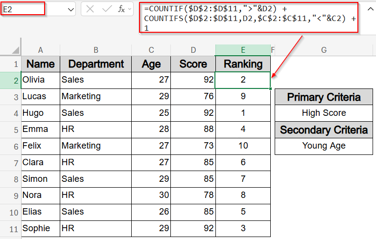
The output ranks every row uniquely based on multiple criteria with no ties unless both criterias have the same value.
Use SUMPRODUCT and COUNTIF Functions for Layered Ranking
This method ranks values by first counting how many Scores are greater using COUNTIF, then adds a tie-breaker by counting how many rows with the exact same Score have a smaller Age using SUMPRODUCT. It’s especially useful for layered ranking logic where you want to handle ties cleanly without helper columns.
For example, if a Score is tied, the formula breaks the tie by assigning a higher rank to the younger individual. This layered approach ensures each record is ranked precisely based on multiple criteria.
Steps:
➤ Click a blank cell like E2 to start.
➤ Type the formula below to rank based on Score and break ties by Age:
=COUNTIF($D$2:$D$11,”>”&D2)+SUMPRODUCT(–($D$2:$D$11=D2), –($C$2:$C$11<C2))+1
This formula counts how many Scores are greater than the current one, then adds how many rows have the same Score but a smaller Age. The “+1” shifts the count into a proper rank.
➤ Press Enter.
➤ Drag the fill handle down to apply the formula to all rows.
This method outputs unique ranks reflecting both Score priority and Age as a tie-breaker which is perfect for multi-level ranking needs.
Create Rankings with RANK and SUMPRODUCT Functions
The RANK function gives each row a rank based on its Score, with higher scores getting better (lower) ranks. To handle ties, we use the SUMPRODUCT function to count how many other rows have the same Score but a younger Age. This helps break ties by ranking older people higher when Scores are equal. The formula combines both checks in one step and gives a unique rank for each row, putting higher Scores first and using Age to decide between ties.
Steps:
➤ Select cell E2 to enter the formula.
➤ Type the following formula to rank by Score and break ties by preferring older ages:
=RANK(D2,$D$2:$D$11) + SUMPRODUCT(–($D$2:$D$11=D2), –(C2<$C$2:$C$11))
➤ Press Enter.
➤ Drag the fill handle down to apply the formula through E11.
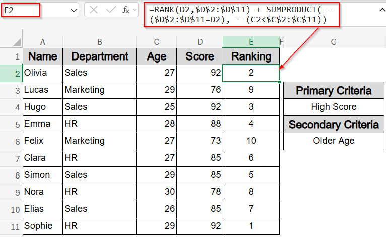
This formula outputs ranks where older individuals are favored among ties, ensuring a fair prioritization based on age.
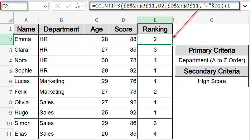
Apply Ranking with RANK and COUNTIFS Functions Using Multiple Criteria
The RANK.EQ function provides the initial rank based on the Score, ranking higher scores better. The COUNTIFS function works as tie-breakers by applying additional criteria: first counting how many tied Scores have a smaller Age, and then among those with identical Scores and Ages, counting how many have a department name that comes earlier alphabetically. This layered use of COUNTIFS function allows sorting by three levels without helper columns, ensuring a strict hierarchical ranking.
In this method, we rank records by Score first, break ties with Age, and finally resolve any remaining ties by sorting departments alphabetically.
Steps:
➤ Click cell E2 to start.
➤ Enter this formula to rank by Score, then Age, then Department:
=IFERROR(RANK.EQ(D2,$D$2:$D$11) + COUNTIFS($D$2:$D$11,D2,$C$2:$C$11,”<“&C2) + COUNTIFS($D$2:$D$11,D2,$C$2:$C$11,C2,$B$2:$B$11,”<“&B2), “”)
➤ Press Enter.
➤ Drag the fill handle down from E2 to E11 to apply it to all rows.
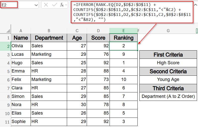
This formula yields unique ranks with a strict hierarchy for Score, Age, and Department, resolving complex ties smoothly.
Ranking Within Groups Using COUNTIFS Function
The COUNTIFS function here counts how many entries within the same Department have a higher Score than the current row. By applying multiple criteria matching Department and comparing Scores, it calculates ranks only within each group rather than across the entire dataset. This targeted ranking helps analyze performance or standings internally within departments.
Steps:
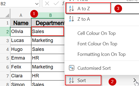
➤ First Sort your data by the order A to Z by right-clicking any cell like B2.
➤ Click cell E2 to enter the formula.
➤ Type the following formula to rank Scores within each Department:
=COUNTIFS($B$2:$B$11,B2,$D$2:$D$11,”>”&D2)+1
➤ Press Enter.
➤ Drag the fill handle down from E2 to E11 to apply it to all rows.
This gives unique ranks within each Department based on Score, allowing focused internal rankings.
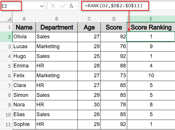
Creating a Combined Decimal Rank Using RANK Function
This method uses two RANK functions separately to rank the data based on Score and Age. The Score rank produces the whole number part, while the Age rank forms the decimal fraction by dividing by 10. Combining them creates a single sortable decimal number that reflects priority by Score first, then Age. This approach is simple and effective for sorting with multiple criteria without complex formulas.
In practice, you rank Scores in one column, Ages in another, and then add them together with the Age rank divided by 10. The result is a combined rank that can be used to sort or filter records based on both criteria simultaneously.
Steps:
➤ In cell E2, type the formula to rank Score column:
=RANK(D2,$D$2:$D$11)
➤Press Enter and drag down using AutoFill from E2 to E11.
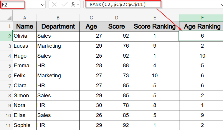
➤ In cell F2, type the formula to find ranking for Age column:
=RANK(C2,$C$2:$C$11)
➤Press Enter and drag down using AutoFill from F2 to F11.
➤ In cell G2, combine the ranks by adding the Score rank to the Age rank divided by 10:
=E2 + F2/10
➤ Press Enter and drag the fill handle down from G2 to G11.
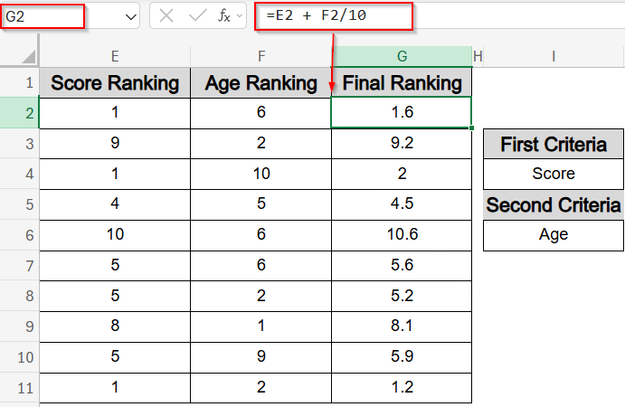
This combined decimal rank helps you quickly sort records by Score and Age in a single column separated by decimal.
Rank Unique Using SUMPRODUCT Function for Multiple Criteria
This method uses the SUMPRODUCT function to assign unique ranks across the entire dataset by comparing both Score and Age simultaneously. It counts how many rows have a higher Score or the same Score but a younger Age, then adds 1 to determine each row’s rank. This approach lets us find the ranking without using RANK and COUNTIF functions.
Steps:
➤ Click cell E2 to enter the formula.
➤ Type the following formula to count entries in the same Score group filtered by smaller Age:
=SUMPRODUCT(($D$2:$D$11>D2) + (($D$2:$D$11=D2)*($C$2:$C$11<C2))) + 1
➤ Press Enter.
➤ Drag the fill handle down from E2 to E11 to apply it to all rows.
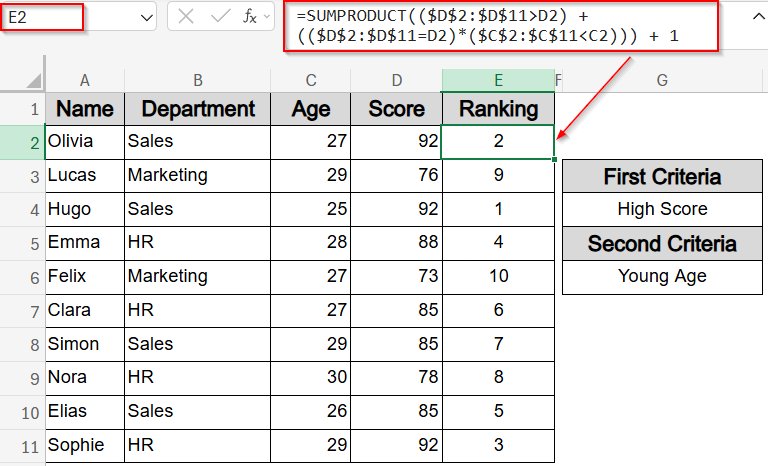
This maintains the higher Score and younger Age hierarchy.
Frequently Asked Questions
Can all formulas handle ties automatically?
Yes, most methods use functions like COUNTIFS or SUMPRODUCT function to break ties by additional criteria, ensuring unique ranks. The approach depends on whether you want to prioritize age, department, or other fields.
Which method is best for ranking within groups?
Methods using COUNTIFS or SUMPRODUCT function with department or group criteria are ideal. They rank data only within each group, giving meaningful comparisons without mixing different categories.
How do I reverse the ranking order?
For descending order, add 1 after a comma in the RANK function like RANK.EQ(value, range, 1). Alternatively, adjust the logic in COUNTIFS or SUMPRODUCT formulas to count lower values instead of higher ones.
Can these formulas be used on large datasets?
Yes, but performance may slow with very large data. Using efficient functions like COUNTIFS helps. For massive datasets, consider Excel’s built-in Sort or Power Query tools for faster processing.
How do I display the rank without gaps?
To avoid gaps, use methods that assign unique ranks like combining COUNTIF and COUNTIFS functions. These count the exact number of entries meeting conditions, ensuring sequential ranks without duplicates or gaps.
Wrapping Up
In this tutorial, we explored eight effective methods to rank data in Excel based on multiple criteria. From simple two-level rankings using RANK and COUNTIFS functions to more advanced approaches with SUMPRODUCT function, you now have flexible tools to handle ties and group-based ranking. Feel free to download the practice file and share your feedback.