When working with data in Google Sheets, you might face cases where numbers are stored as text. This can cause problems with calculations and data analysis. That means you can’t use them for calculations until you convert them.
That’s why Google Sheets provides several simple ways to convert text to numbers. In this article, we’ll learn some easy techniques to convert text to real numbers in Google Sheets. These methods are simple and do not need any special skills.
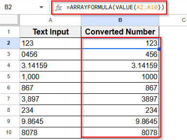
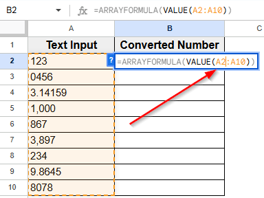
Here is a step-by-step guide to apply ARRAYFORMULA function to convert text to number in Google Sheets:
➤ Click on the first cell of Column B that is next to A2 cell.
➤ In B2 cell, type the formula =ARRAYFORMULA(VALUE(A2:A10)). We include A2 to A10 in the formula because we want to convert all the text to numbers in those cells.
➤ Press Enter.
➤ This formula will now convert all the values in Column A into numbers and display them in Column B.
Using the VALUE Function
The easiest way to convert text to numbers in Google Sheets is using the VALUE function. It takes a text entry that looks like a number and turns it into a real, usable number. You can then apply formulas like SUM, AVERAGE, or other calculations without any issues.
Here’s how you can use the VALUE function:
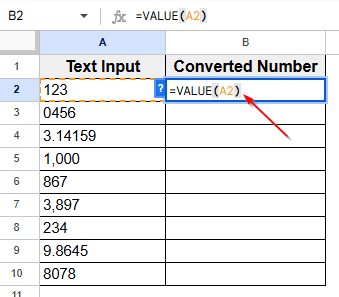
➤ Click on the first cell in Column B which is next to the text number in A2 cell.
➤ In B2 cell type this formula:
=VALUE(A2)
This formula tells Google Sheets to take the text in cell A2 and convert it into a real number.
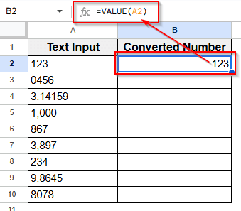
➤ Press Enter. Now you’ll see the actual number appear in cell B2.
➤ Next, drag down the small blue dot of the square which is at the bottom-right corner of the cell to apply this formula to the entire column.
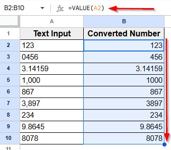
It looks the same as before, but now it’s a number that you can use in calculations.
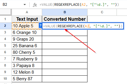
Applying REGEXREPLACE with VALUE Function
If a cell has both numbers and other characters, you can use REGEXREPLACE to keep only the numbers, then use the VALUE function to turn it into a real number. This method is helpful when your data includes things like words, commas, or currency signs. The formula cleans it up so you can use the number in calculations.
Here is how you can apply this formula:
➤ Select cell B2 and type the following formula:
=VALUE(REGEXREPLACE(A2, "[^\d.]", ""))
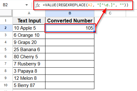
➤ Press Enter and you’ll see the number appear without the extra text or symbols. This formula removes everything from A2 that is not a number or a dot.
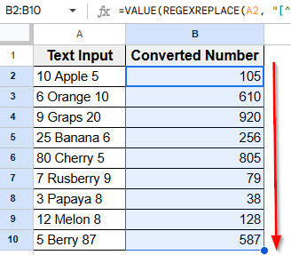
➤ Drag the fill handle down to apply the formula to the rest of the column.
Inserting ARRAYFORMULA Function for Bulk Conversion
If you want to change a whole column of text numbers to real numbers all at once, you can use ARRAYFORMULA. This lets you apply one formula to many cells without copying it down one by one.
Here is a step-by-step guide to apply this formula:
➤ Click on the first cell of Column B that is next to A2 cell.
➤ In B2 cell, type the following formula. We are including A2 to A10 as the cell range inside the formula because we want to convert all the text to numbers in those cells.
=ARRAYFORMULA(VALUE(A2:A10))
➤ Press Enter.

➤ This formula will now convert all the values in Column A into numbers and display them in Column B.
Now you don’t have to drag anything like previous methods, the formula automatically applies to all rows in that range.
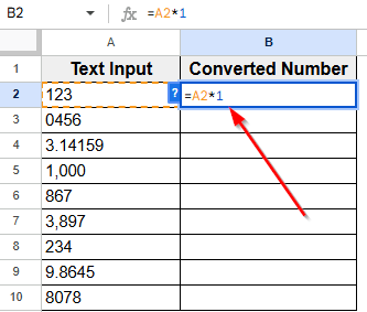
Multiplying by 1 to Convert Text to Number
This is one of the fastest and easiest ways to turn text into numbers in Google Sheets. When you multiply a text number by 1, Google Sheets automatically treats it as a real number.
Here is you can apply this function:
➤ Click on the first empty cell in Column B that is next to A2 cell.
➤ Type this formula in cell B2:
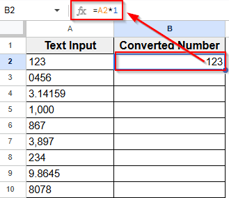
=A2*1
➤ Now, press Enter. You’ll see the text value of A2 cell converted to the real number in the B2 cell.
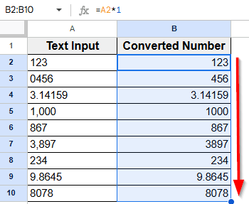
➤ Drag the blue dot or fill handle down to copy the formula to the other rows in Column B.
Frequently Asked Questions
How to convert word to number in Google Sheets?
Sometimes, a number is stored as text in a cell. For example, you might see “123” in a cell, but Google Sheets treats it like a word, not a number. This can stop your formulas from working.
To fix it, you can use the VALUE function. Type this formula in another cell: =VALUE(A2) and click Enter. It will convert text into the real number.
How do I get a numeric value from a string in Google Sheets?
To do this, you can use the REGEXREPLACE function to keep only the numbers, and then use VALUE to turn it into a real number. Type this formula into B2 cell: =VALUE(REGEXREPLACE(A12, “[^\d.]”, “”)) and then click Enter.
Wrapping Up
Converting text to numbers in Google Sheets helps your data work properly. If numbers are stored as text, your formulas might not work, and your results could be wrong. It can also cause problems when you try to add numbers, make charts, or sort data.
Google Sheets offers some powerful formulas that can save you time and hassle. These formulas turn text into real numbers, so you can do calculations, create charts, and analyze data without any trouble.