Gridlines in Google Sheets is a useful feature that allows users to view and align their data or elements. However, it can be distracting when you are trying to present your data in a clean, professional format. Removing gridlines helps users to better organize data and focus attention on specific sections. Although there are no built-in tools in Google Sheets that allow users to remove gridlines from specific cells, there are many workarounds.
To remove gridlines from specific cells in Google Sheets, follow the steps below:
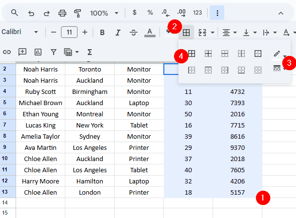
➤ Select the cell or range of cells where you want to hide the gridlines.
➤ Next, click on the Borders icon from the toolbar, then select Border color and set it to white.
➤ Finally, select All Borders from the Borders menu to apply white borders to the range of cells.
In this article, we will learn 3 effective methods of removing gridlines from specific cells in Google Sheets.
Remove Gridlines from Specific Cells Using Custom Borders
This is the simplest and easiest method of removing gridlines from specific cells in Google Sheets. This method involves the use of Border tool to remove gridlines from specific cells in a spreadsheet file.
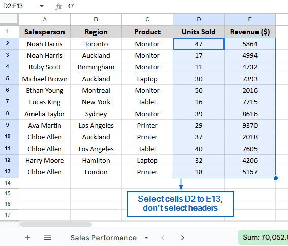
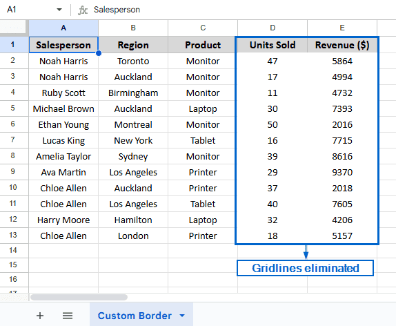
In the sample dataset, we have a worksheet called Sales Performance containing information about Salesperson, Region, Product, Units Sold and Revenue. By using custom borders, we will eliminate all gridlines from columns D and E, containing information about Units Sold and Revenue. The updated spreadsheet with hidden gridlines will be stored in a separate worksheet called “Custom Border”.
Steps:
➤ In the Sales Performance worksheet, select the range of cells D2:E13 to include all elements of columns D and E except for the headers.
➤ Next, from the toolbar, head to Borders option, change the Border color to White and click on All borders.
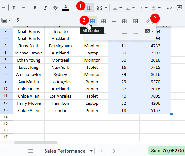
➤ Columns D and E should be free of gridlines now.
Remove Gridlines from Specific Cells Using Custom Apps Script
Google Apps Script is a very powerful tool that lets users automate and customize tasks in Google Sheets. We can also remove gridlines from specific cells using this tool. This method is ideal for users who want to complete the operation without manually adjusting borders or sheet settings. Unlike the first method, this method is more time-efficient and can be applied to the entire dataset all at once. We will work with the same dataset and use a custom Apps Script to remove gridlines from columns D and E. The new updated dataset will be stored in the “Apps Script” worksheet.
Steps:
➤ Open the Sales Performance worksheet and head to Extensions >> Apps Script.

➤ In the script editor, paste the following code:
function hideGridlinesFromSpecificColumns() {
  var sheet = SpreadsheetApp.getActiveSpreadsheet().getActiveSheet();
  var range = sheet.getRange("D2:E13");
  range.setBorder(true, true, true, true, true, true, "white", SpreadsheetApp.BorderStyle.SOLID);
  range.setBackground("white");
}
Note:
In the custom script,
➧ function hideGridlinesFromSpecificColumns() part defines the function that will be used to hide gridlines in the column.
➧ var sheet = SpreadsheetApp.getActiveSpreadsheet().getActiveSheet(); recalls the currently active spreadsheet where the script will be executed.
➧ var range = sheet.getRange(“D2:E13”); it defines the range of cells from D2 to E13 where we want to remove the gridlines.
➧ range.setBorder(true, true, true, true, true, true, “white”, SpreadsheetApp.BorderStyle.SOLID); this is the part that applies a white border on all sides of the selected range of cells.
➧ range.setBackground(“white”); this line fills the selected range of cells with white background color.
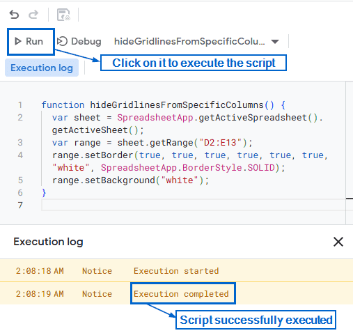
➤ Next, click on Run from the script editor menu and wait for the script to execute.
Note:
Once the script runs successfully, the execution log will show the message “Execution completed”.
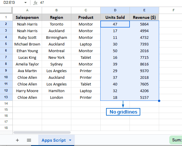
➤ Lastly, head to the Apps Script worksheet, and you will see all the gridlines from columns D and E have been successfully removed.
Remove Gridlines from Specific Cells Using Menu Bar Options
We can remove gridlines from specific cells or columns using Google Sheets’ main menu as well. Unlike the first two methods, this method is more straightforward but takes longer to execute since it involves manually adding and removing gridlines across the entire spreadsheet file. We will again work with the same dataset and display the modified file in separate “Main Menu” worksheet.
Steps:
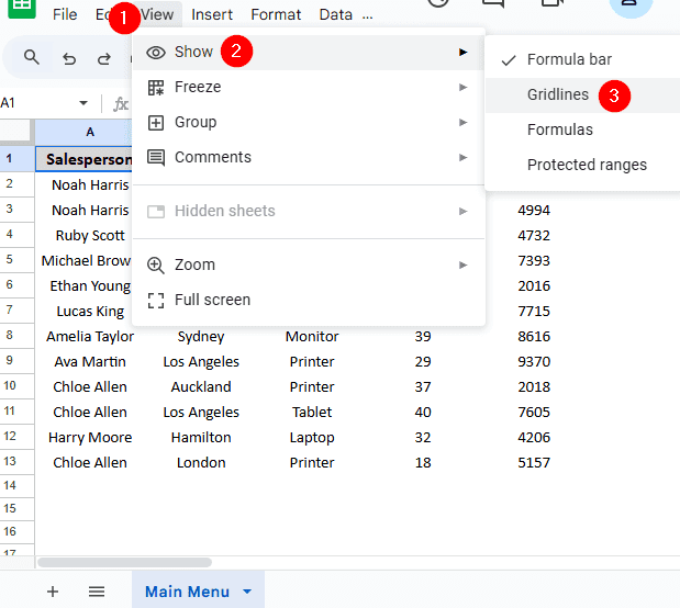
➤ Open the Sales Performance worksheet, head to View >> Show and uncheck the Gridlines box. The entire dataset should now have gridlines removed.
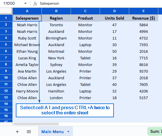
➤ Next, click on cell A1 and press Ctrl + A twice. This should select the entire dataset.
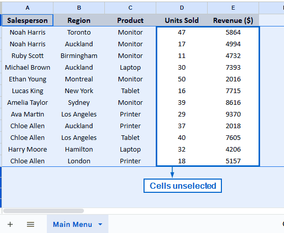
➤ Now, pressing Ctrl , move your cursor and select all cells of columns D and E except for the header. This should unselect the cells in columns D and E.
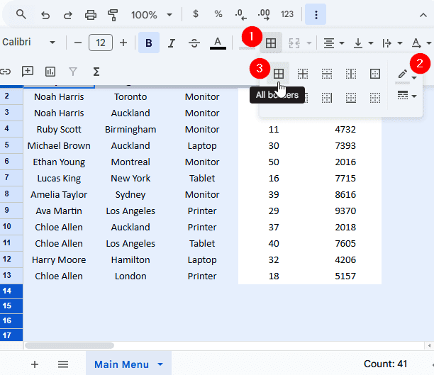
➤ Then, go to the toolbar and click on the Borders icon. From the dropdown menu, set the Border colour to Grey and select All Borders.
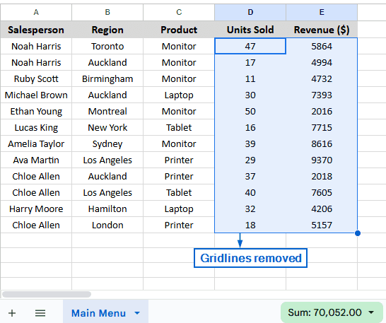
➤ You should now have a dataset where gridlines are hidden in columns D and E.
Frequently Asked Questions
Which Method Should I Use For Working With Large Datasets?
If you are working with large datasets, it is best to use the Apps Script method. The Apps Script method automates the gridline removal process, saving time and improving efficiency.
Will Removing Gridlines Affect My Data or Formula?
Removing gridlines following any of the methods discussed in this article will not affect your data, formula or cell references.
Concluding Words
Removing gridlines from specific cells or columns in Google Sheets is essential for enhancing data visualization and presentation. In this article, we have discussed 3 efficient methods of removing specific gridlines by using Custom borders, Apps Script and the Main menu. Feel free to try out every method and choose one that is best suited for your needs.