Both sorting and filtering help you arrange a large database according to specific criteria. While both functions help in organizing data, they serve different purposes. Sorting helps you alphabetize, rank data, and maintain chronological order. Filtering allows you to select specific data matching a certain criterion and change it according to your needs.
In Excel, sorting and filtering methods are strikingly different, each offering single, multilevel, and custom alterations of your dataset.
Some key differences between sorting and filtering in Excel include:
➤ Sorting arranges data in a structured way (e.g., alphabetical, numerical, or custom order). Filtering focuses on specific subsets of data without altering the original arrangement.
➤ While sorting is used for grouping values in a logical order, filtering is used to quickly separate values based on a criteria match.
➤ You can sort data alphabetically, numerically, by multiple columns, and by dates, numbers, colors, or icons. Custom sorting allows you to sort by your defined list
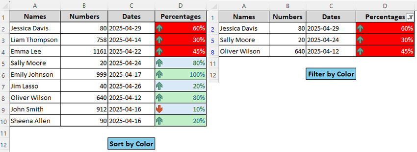
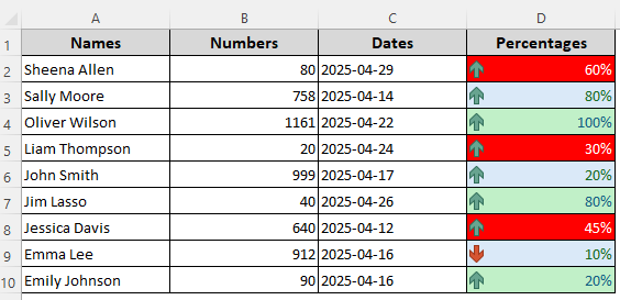
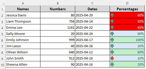
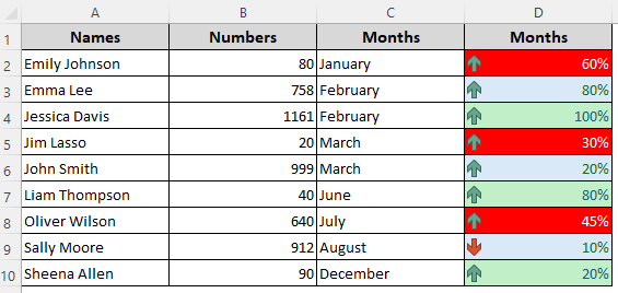
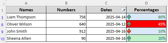
➤ Similarly, common filtering methods include filtering by texts, numbers, dates, columns, colors, or icons. Advanced filtering lets you filter data based on custom criteria or a list you specify. The following image shows a dataset sorted and filtered by the color Red in Column D.
In this article, we’ll explore all the differences between sorting and filtering, from their definitions to application and methods with practical examples.
Definition of Sorting and Filtering in Excel
Let’s start by understanding what the terms sort and filter mean in Excel. Here’s the difference in their definitions:
What Is Sorting?
In Excel, sorting means arranging data in a specific order—either ascending (A to Z or smallest to largest) or descending (Z to A or largest to smallest). You can apply it to multiple columns containing texts and numbers.
What Is Filtering?
Filtering means displaying only the rows or columns that meet certain criteria and hiding the others. Unlike sorting, filtering doesn’t rearrange your data. It temporarily blocks out specific data and brings the hidden data back once the filter is cleared.
Uses of Excel’s Sort and Filter Features
Usually, sort and filter features are used for data organization and analysis. While sorting arranges your data logically, filtering helps you focus on specific information without removing anything. Below are the differences between the usage of each feature:
Sorting Is Used For:
- Organizing data alphabetically (A–Z or Z–A)
- Arranging numbers from smallest to largest or vice versa
- Sorting by date, from oldest to newest or newest to oldest
- Sorting based on cell or font color
- Prioritizing tasks or entries based on status or ranking
- Easily compare related data points by grouping similar items
Filtering Is Used For:
- Viewing only rows that meet specific criteria like showing only completed tasks
- Quickly finding values or text within large datasets
- Hiding rows without deleting them
- Filtering based on multiple conditions (e.g., Numbers >=50 AND Names = “Liam”)
- Isolating duplicates, blanks, or specific text matches
- Analyzing subsets of data without changing the original layout
- Using custom filters for advanced analysis (like top 10 items or dates between ranges)
Examples of Sorting Data in Excel
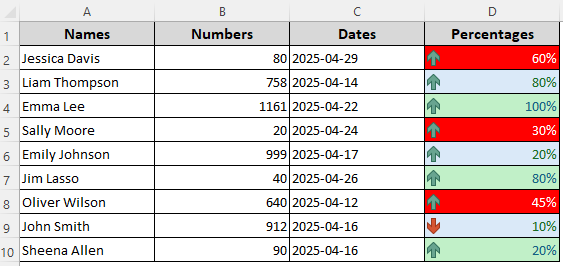
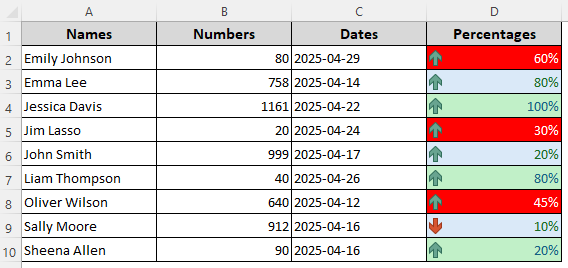
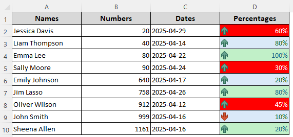
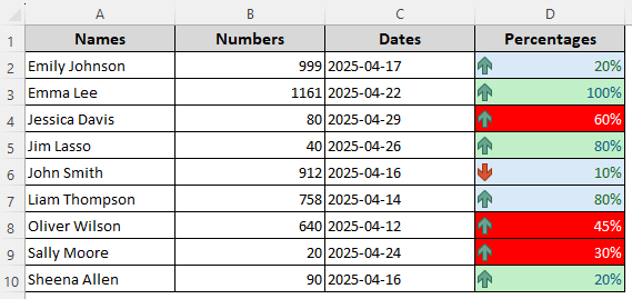
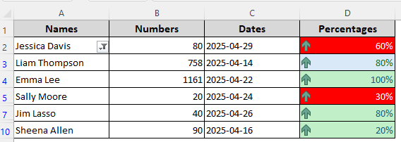
To explore the different sorting methods, we’ll use the following dataset containing columns with random names, numbers, dates, etc. With this data, we’ll explain the different sorting methods.
Column D has data in different font colors, conditional formatting icons, and fill colors to explain certain sorting and filtering methods. Keep in mind that sorting will rearrange your data, so you must choose the entire dataset or expand the selection for related columns and rows.
Sorting Data Alphabetically
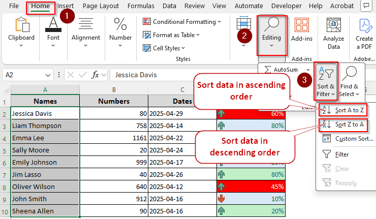
➤ Select the data range you want to sort (without the headers) and go to the Home tab.
➤ From the Editing tab, select Sort & Filter.
➤ To sort data in an ascending order, click on Sort A to Z.
➤ Choose the Sort Z to A option to arrange data in a descending order.
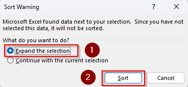
➤ If prompted, choose Expand the Selection and press Sort to keep related data intact.
➤ Here’s the result for ascending order:
➤ Here’s the result for descending order:
Sorting Data Numerically
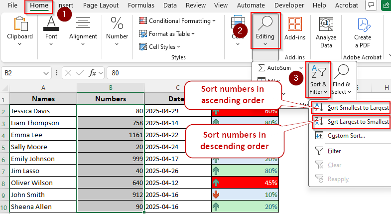
➤ Highlight the data range with numeric values and go to the Home tab.
➤ Choose Sort & Filter from the Editing group.
➤ Click on Sort Smallest to Largest to rearrange data in an ascending order (1 to 100).
➤ Select Sort Largest to Smallest to rearrange the numbers in a descending order (100 to 1).
➤ Expand the selection if necessary.
➤ Our final result for ascending order is as follows:
➤ Our final result for descending order is as follows:

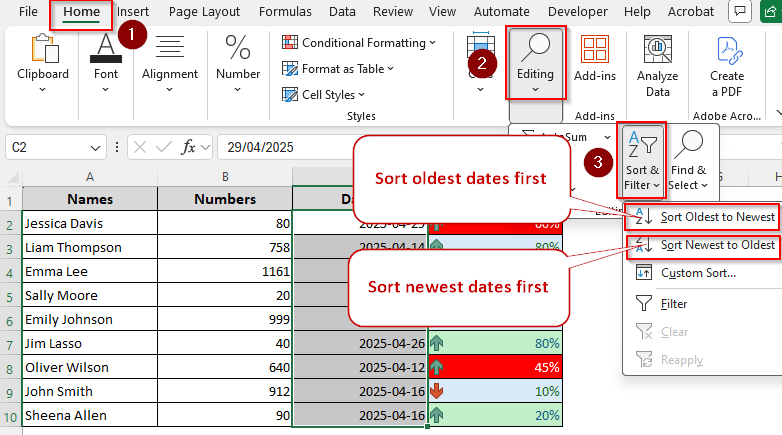
Sorting by Date
➤ Select the data with dates and go to the Home tab.
➤ Click on Sort & Filter in the Editing group.
➤ To sort old dates at the top, select Sort Oldest to Newest.
➤ Choose Sort Newest to Oldest to rearrange the dates starting from the newest one.
➤ If needed, select the Expand the Selection option when prompted.
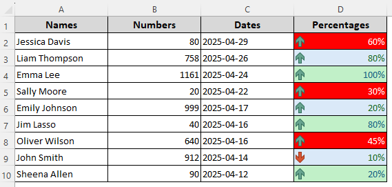
➤ Sorted dates in an ascending order should be like this:

➤ Sorted dates in a descending order should be like this:
Sorting by Cell Color, Font Color, or Icon
➤ Select your data range (without the headers) and open the Home tab >> Sort & Filter >> Custom Sort.
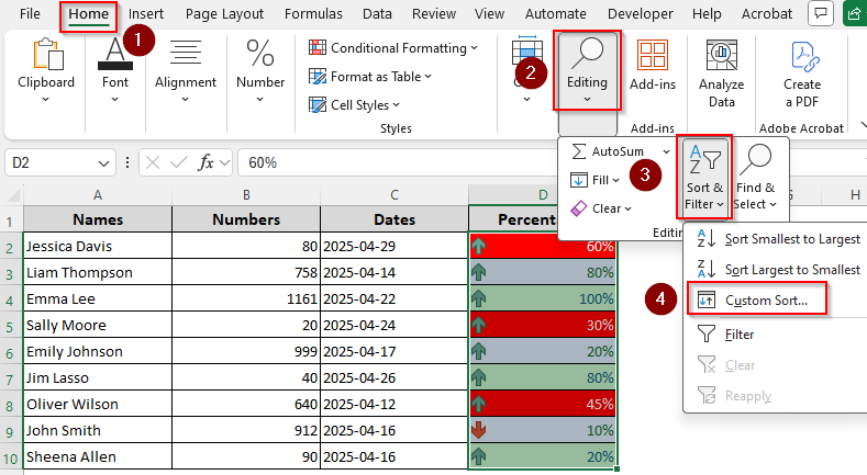
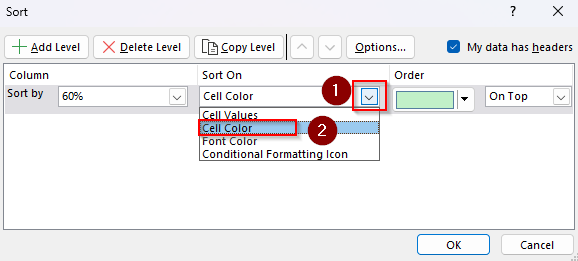
➤ From the Sort dialog box, click the Sort On drop-down and choose Font Color, Cell Color, or Conditional Formatting Icon based on your data type and desired results. We selected Cell Color to sort based on the fill colors of the cells.
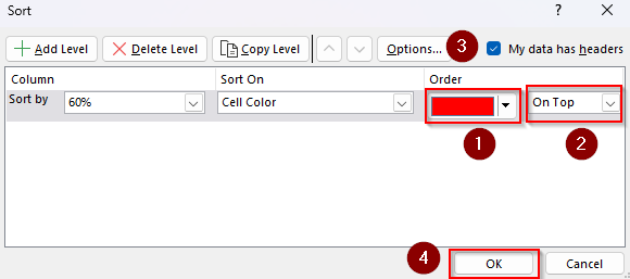
➤ Now, click on the Order drop-down and select the color you want to sort by. We chose the red color.
➤ Choose whether you want to keep the cells On Top or On Bottom.
➤ Finally, check the My Data Has Headers box and press Ok.
➤ Here’s the final result:
Multi-Level Sorting
➤ To sort data based on multiple criteria (e.g., first by names, then by dates), select the data range. Go to the Home tab >> Sort & Filter >> Custom Sort.
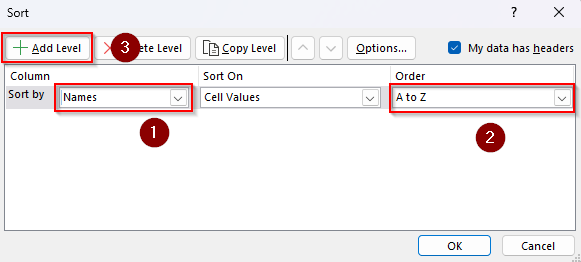
➤ In the Sort dialog box, click the Sort By dropdown and choose the first column (first level) you want to sort by.
➤ From the Order drop-down, choose the sort order such as A to Z or Smallest to Largest.
➤ Press the Add Level button at the top to add another sorting criterion.
➤ From the Then By drop-down, select the second column to sort by. Click on the Order drop-down to rearrange the data in ascending or descending order.
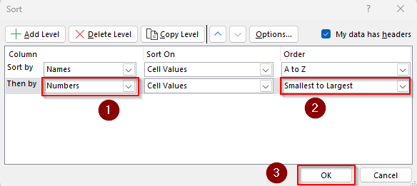
➤ Finally, click Ok to apply the multi-level sort.
Custom Sorting by User-Defined Order
➤ This time we’ll sort a list of months. To sort data based on a predefined list, select the data range and click on the Home tab >> Sort & Filter >> Custom Sort.
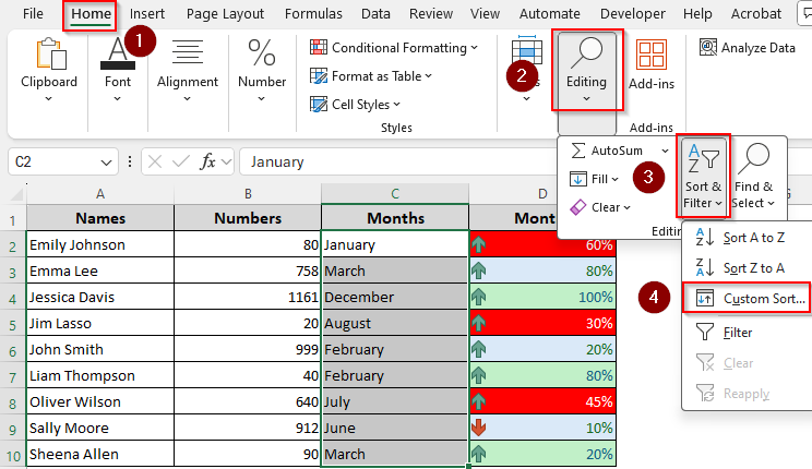
➤ In the Sort By dropdown, choose the column you want to sort.
➤ From the Order drop-down, select Custom List.
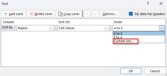
➤ Enter your list with commas or select Excel’s predefined list like the Days of the Week or Months of the Year. Click Ok.
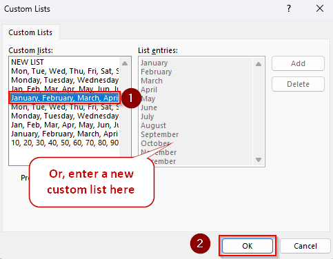
➤ Press Ok to get the sorted data.
Examples of Filtering Data in Excel
We’ll use the same dataset to apply different filtering methods. As filtering works on the entire row or column, make sure you select the correct range for related data in different rows and columns.
Basic Filter (AutoFilter)
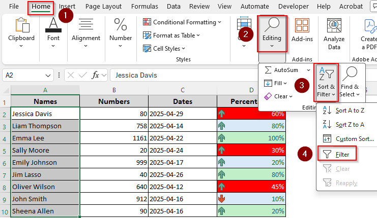
➤ Select your data range and go to the Home tab.
➤ From the Editing group, click on Sort & Filter. Select Filter from the menu.
➤ As Excel adds a drop-down in the header cell(s), click on it and review the list of options.
➤ Now, uncheck all the boxes containing the values you want to filter out or hide temporarily.
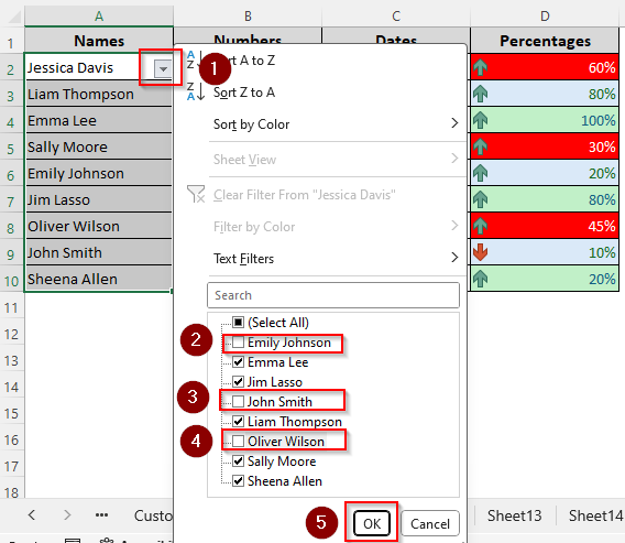
➤ Press Ok and Excel will display only the data from the checked boxes. You can make the necessary changes in this filtered data.
➤ To remove the filter and bring back your original data, go to the Home tab >> Sort & Filter >> Filter.
Filtering by Text
➤ To filter texts based on specific conditions, select your data range and open the Home tab >> Sort & Filter >> Filter.
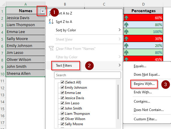
➤ Click on the drop-down arrow on the column heading and choose Text Filters.
➤ Depending on your desired result, you can choose any of the given options to filter text that Equals/Does Not Equal, Begins With, Ends With, Contains/Does Not Contain certain letters or words.
➤ For example, we’ll filter names starting with the letter S. So, we click on Begins With.
➤ As the Custom AutoFilter dialog box appears, enter S in the empty field beside Begins With.
➤ For more customization, you can click the And/Or option and add more letters or texts.
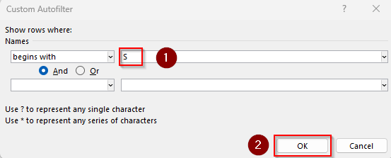
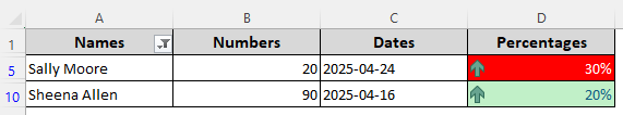
➤ Click Ok and Excel will now display only names starting with S.
Filtering by Number
➤ Select numbers to filter and click on the Home tab >> Sort & Filter >> Filter.
➤ On the column header, press the drop-down arrow and choose Number Filters from the menu.
➤ Depending on your desired result, choose from the given criteria, including Equals/Does Not Equal, Greater Than/Less Than, Greater/Less Than Or Equal To, Between, Top 10, Above/Below Average.
➤ As we click on the Greater Than Or Equal To option, the Custom AutoFilter box opens.
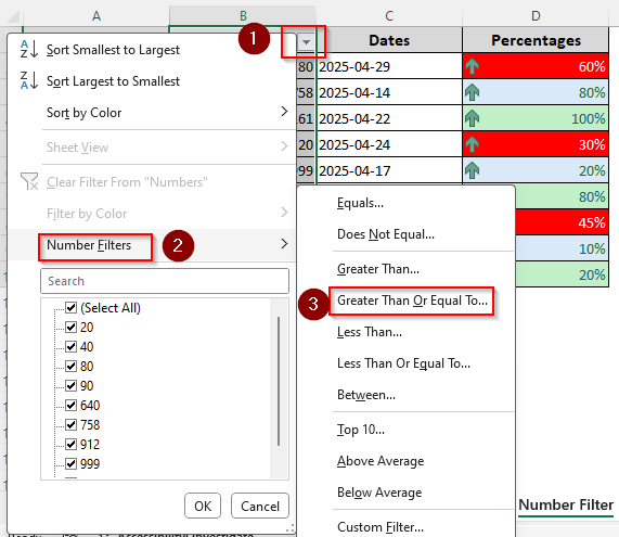
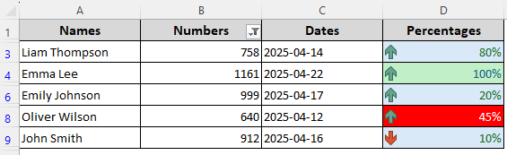
➤ In the Is Greater Than Or Equal To field, manually type a number or select one from the drop-down.

➤ Press Ok and Excel will only display numbers meeting the criteria.
Filtering by Date
➤ Start by selecting the dates you want to filter and go to the Home tab >> Sort & Filter >> Filter.
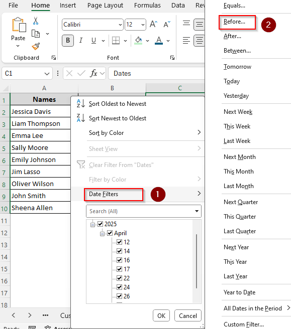
➤ Click on the filter drop-down on the column header and choose Date Filters.
➤ From the menu, choose your desired filter from the given options, including Equals, Before, After, Between, Tomorrow, Today, Yesterday, Next Week, This Week, Last Week, Next Month, This Month, and Last Month.
➤ We selected the Before option to filter days before 2025-04-17.
➤ As you click on the criteria, the Custom AutoFilter dialog box opens. In the Date field, manually type a date or choose one from the drop-down to filter by that date.
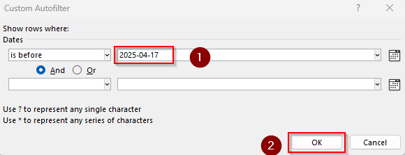
➤ Press Ok and your data will be filtered accordingly.
Filter by Cell Color/Font Color/Icon
➤ Select your data range and open the Home tab >> Sort & Filter >> Filter.
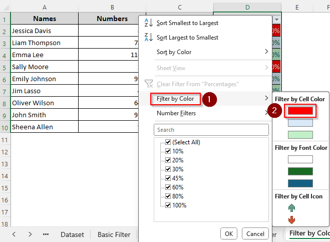
➤ Click on the drop-down arrow sign on the column heading. Choose Filter By Color from the given options.
➤ Depending on your filter criteria select Filter By Cell Color, Filter By Font Color, or Filter By Cell Icon.
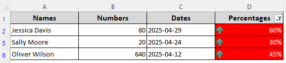
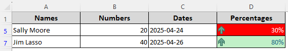
➤ Finally, choose the specific cell color, font color, or icon you want to filter by. We’ll filter by cell color and filter cells with red fill color.
➤ Press Ok to see the filtered data.
Advanced Filter (User-Defined Criteria)
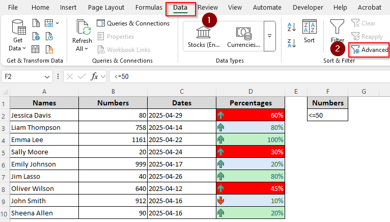
➤ First, set up a criteria range to use for filtering. You can create a list or use a single cell. For example, we’ll enter <=50 in cell F2 to filter numbers less than or equal to 50.
➤ Make sure the criteria cell/range has the same heading as the column containing the data you want to filter as we entered the heading in cell F1.

➤ Now, select the data you want to filter and go to the Data tab. From the Sort & Filter group, select Advanced.
➤ In the Advanced Filter dialog box, choose Filter the List, In-Place from the Action group.
➤ Excel will now automatically select your data range and display it in the List Range field. If it doesn’t or selects the wrong dataset, you can select it manually. Make sure you include the header.
➤ In the Criteria Range field, highlight the criteria range from your dataset including the header. We’re selecting the cells F1 and F2.
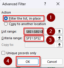
➤ Press Ok to see the filtered data.
Sorting VS Filtering at a Glance
The following table explores the key differences between sorting and filtering in short.
| Topic | Sort | Filter |
|---|---|---|
| Purpose | Rearranges data in order | Displays only matching data |
| Effect | Rearranges all rows | Hides non-matching rows |
| Data Visibility | All data remains visible | Only filtered data is visible |
| Methods | Sort in ascending and descending orders, sort by numbers, texts, dates, colors, or custom conditions | Filter specific values, filter by texts, numbers, dates, colors, and custom criteria |
| Uses | Alphabetize, rank, chronological order | Hide irrelevant info, compare filtered subsets, search within columns, group similar categories |
| Advantages | Organize a huge dataset at once, change data order in a few clicks based on custom conditions | Quickly find blanks, duplicates, and other data errors, make changes in filtered subsets without affecting the original data |
Frequently Asked Questions
How to use the SORT function in Excel?
Excel’s SORT function allows you to dynamically sort data in Excel without changing the original dataset. For example, to sort the range A2:D10 based on the second column in ascending order, enter the following formula in a helper column cell:
=SORT(A2:D10, 2, 1)
Change the data range A2:D10, column number 2 to sort by, and order 1 (use 2 for descending order) according to your dataset.
What is the difference between sort and sort by in Excel?
The sort feature (Home tab >> Sort & Filter >> Sort) lets you sort your data by one or more columns manually. This single-level sorting is useful for quick sorting in-place. On the other hand, the sort by feature (Home tab >> Sort & Filter >> Sort >> Sort dialog box) allows multi-level sorting based on multiple columns. It’s useful to organize large data sets with multiple criteria.
What is the FILTER function in Excel?
The FILTER function allows you to extract a subset of data that meets certain conditions. For example, to return only the rows from A2:D10 where column B contains 50, insert the following formula in a helper column cell:
=FILTER(A2:D10, B2:B10=50)
Change the filter range A2:D10, lookup range B2:B10, and lookup value 50 according to your needs.
Concluding Words
Sorting is for rearranging data order while filtering is to extract specific data based on a specific condition. Both features have numerous uses in Excel from ranking data to quickly deleting repetitive or unnecessary values in bulk. For organized and powerful data analysis, you can combine sorting and filtering for specific requirements.