
Merging multiple columns in Excel is a common task, especially when combining data like full names or addresses that are split across separate columns. Although Excel has no direct tools that allow users to do this, we can use several alternative methods to achieve the same result.
Follow the steps below to merge 3 columns in Excel:
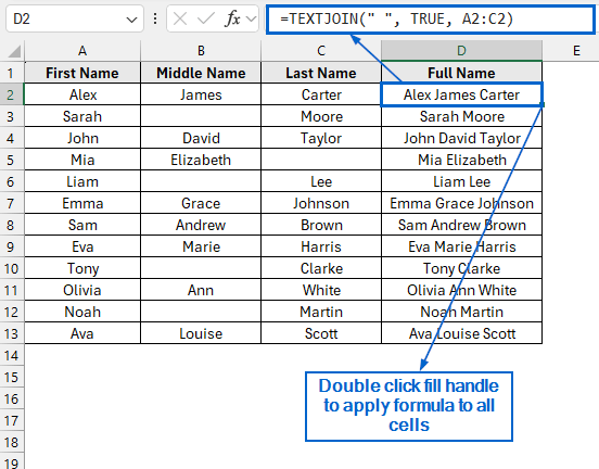
➤ In your dataset, select the cell where you want to display the merged result and put the formula:
=TEXTJOIN(” “, TRUE, A2:C2)
➤ Replace A2:C2 with the range of cells that you want to merge.
➤ Press Enter, then double click the fill handle to apply formula to the rest of the column.
In this article, we will learn six effective methods of how to merge 3 columns in Excel.
Combine Columns Easily Using the TEXTJOIN Function
In the sample dataset, we have a worksheet called Names containing information about First Name, Middle Name and Last Name of employees. By using the TEXTJOIN function, we will merge the First Name, Middle Name, and Last Name columns into a single Full Name, which will then be displayed in column D of the dataset. We will show the modified dataset in a separate TEXTJOIN Function worksheet.

The TEXTJOIN in Excel is a simple function that is used to combine multiple text values from different cells or ranges into one single text string, with a custom delimiter between them.
Steps:
➤ Open the TEXTJOIN Function worksheet and in cell D2, put the following formula:
=TEXTJOIN(" ", TRUE, A2:C2)
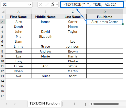
➧ TEXTJOIN is used to combine the text from multiple cells into one cell.
➧ " " uses space as a separator to separate the text from each cell.
➧ TRUE part tells the formula to ignore any empty cells in the range.
➧ A2:C2 is the range of cells whose data we want to join.
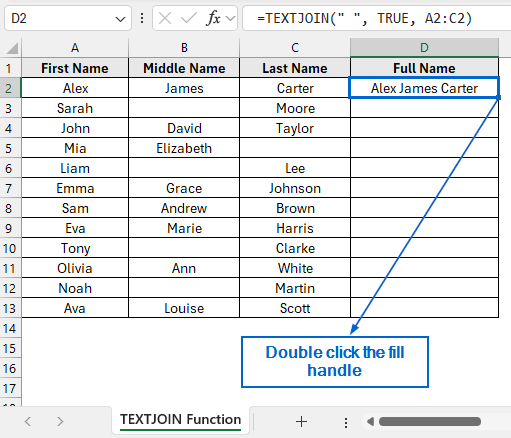
➤ Next, select cell D2 again and double click the fill handle to apply the formula across column D.
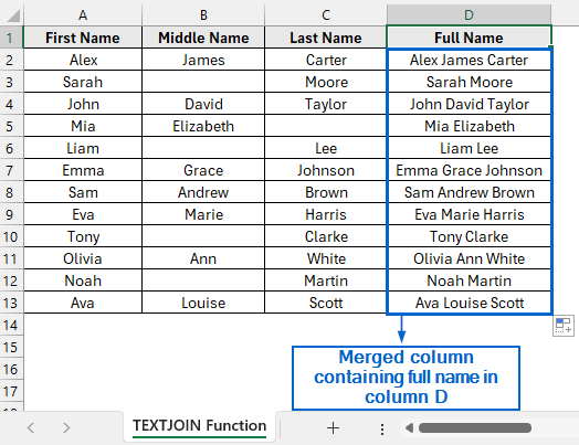
➤ The merged column containing the Full Name of the employees should now be visible in column D.
Merge Columns with Ampersand (&) and IF Function
The Ampersand (&) is a simple operator in Excel used to join text strings together. On the other hand, the IF function allows users to perform logical comparisons between values. By combining these two tools, we can easily merge data from 3 columns into a single column in Excel.
We will work with the same dataset and use Ampersand (&) with IF Function to display the merged full name in column D of the dataset. The updated dataset will be stored in a separate worksheet called Ampersand with IF Function.
Steps:
➤ Open the Ampersand with IF Function worksheet and in cell D2, put the following formula:
=A2 & IF(B2<>"", " " & B2, "") & IF(C2<>"", " " & C2, "")
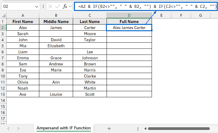
➧ A2 part takes the value from cell A2.
➧ IF(B2<>"", " " & B2, "") checks whether cell B2 is not empty. If it contains data, it adds a space " " followed by the value in B2. If B2 is empty, no extra space or text is added.
➧ IF(C2<>"", " " & C2, "") does the same thing as before for cell C2.
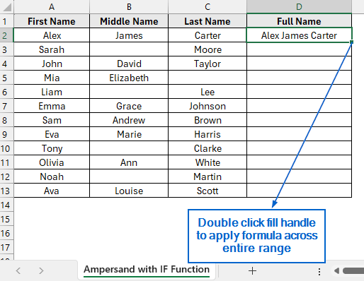
➤ Then, select cell D2 again and double-click the fill handle to apply the formula across the entire range.
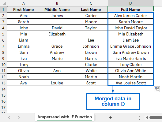
➤ You should now see the merged data being displayed in column D.
Use Power Query to Automatically Merge Columns
Power Query in Excel is a powerful tool allowing users to import, transform, and clean data from various sources efficiently. We will again work with the same dataset, and this time use Power Query to display merged data in column D of the dataset. We will display the updated dataset in a separate Power Query worksheet.
Steps:
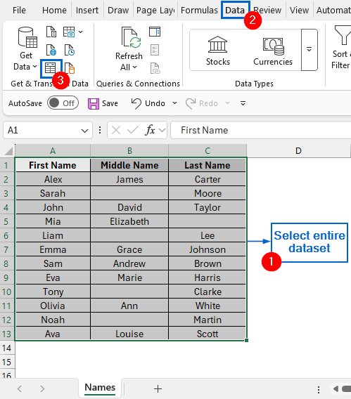
➤ Open the Names worksheet, select the entire dataset and from the Data tab, click on From Table/Range.
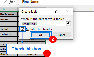
➤ Check the “My table has headers” box in the Create Table pop-up menu, then click OK.
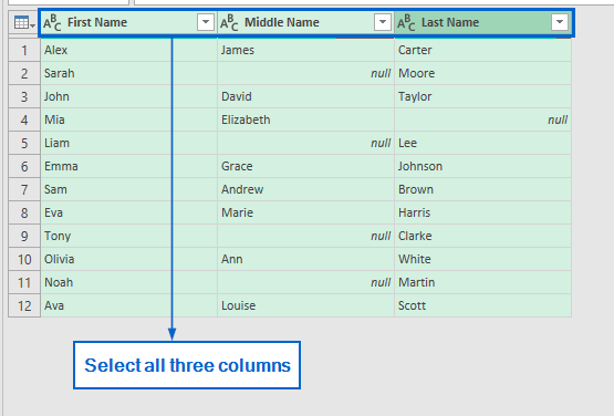
➤ In the Power Query Editor, press Ctrl and select all three columns.
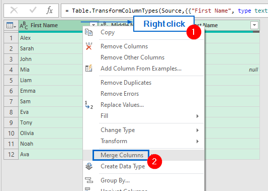
➤ Then, Right-click on any of the selected columns and choose Merge Columns from the context menu.
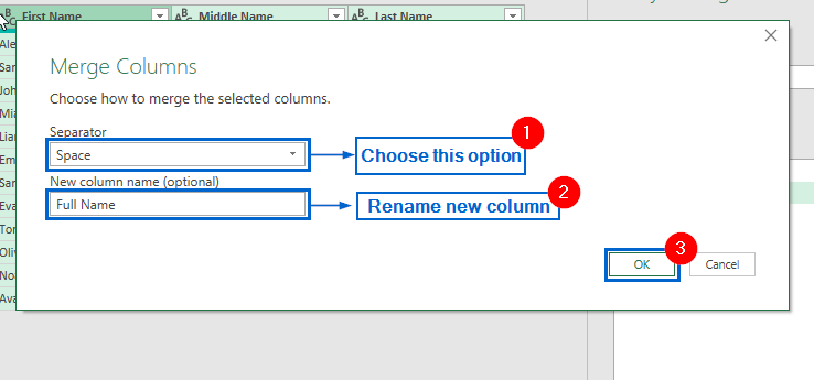
➤ In the Merge Columns dialogue box, select Space as the separator, enter “Full Name” as the new column name, and click OK.
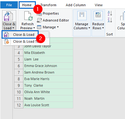
➤ Lastly, head to Home tab and click Close & Load to complete the operation.
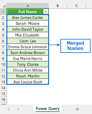
➤ Merged names should now be displayed in the worksheet.
Concatenate Columns Using CONCATENATE Function
Similar to Ampersand (&), the CONCATENATE function combines text or values from multiple cells into one, allowing users to combine data from multiple columns into a single column.
Working again with the same dataset, we will combine names and use the CONCATENATE function to display the merged value in column D of the dataset. The modified dataset will be displayed in a separate CONCATENATE Function worksheet.
Steps:
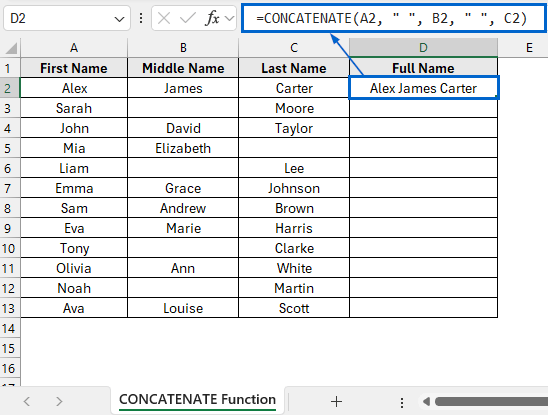
➤ Open the CONCATENATE Function worksheet and in cell D2, put the following formula:
=CONCATENATE(A2, " ", B2, " ", C2)
Note:
This simple formula takes the values from cells A2, B2, and C2, and combines them by adding a space between them.
➤ Then, select cell D2 again and apply formula to the remaining cells by double-clicking the fill handle.
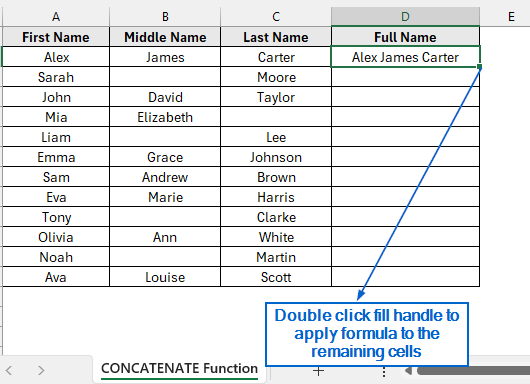
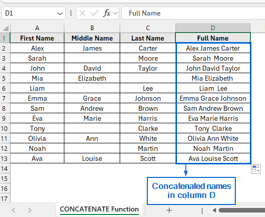
➤ Column D should now display the concatenated names.
Combine Columns Using CONCAT and IF Functions
Both the CONCAT and CONCATENATE functions can perform similar tasks, but the CONCAT function offers more flexibility and enhanced functionality. Unlike CONCATENATE, CONCAT can be combined more effectively with conditional logic like IF, to allow users to merge values dynamically based on specific conditions.
Again, working with the same dataset, we will use both CONCAT and IF functions to combine the name columns and display them in column D of the dataset. The updated dataset will be displayed in a separate CONCAT with IF Function worksheet.
Steps:
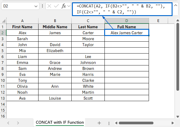
➤ Open the CONCAT with IF Function worksheet and in cell D2, put the following formula:
=CONCAT(A2, IF(B2<>"", " " & B2, ""), IF(C2<>"", " " & C2, ""))
➧ A2 part inserts the value from cell A2.
➧ IF(B2<>"", " " & B2, "") checks if cell B2 is not empty. If it is not, it adds a space followed by the value in B2; if it is empty, it adds nothing.
➧ IF(C2<>"", " " & C2, "") does the same thing, but for cell C2.
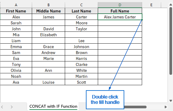
➤ Then, again select cell D2 and apply the formula to the remaining cells by double clicking on the fill handle.
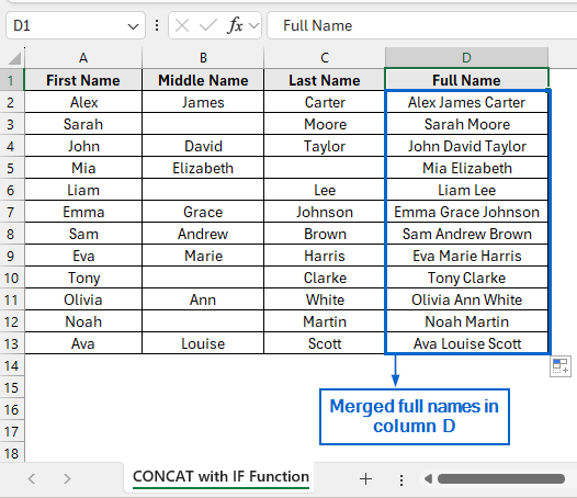
➤ The merged full name should now be visible in column D of the dataset.
Use LET Function for Efficient Merging
The LET function in Excel allows users to assign names to calculation results and reuse them in a formula. Unlike other methods that repeat the same logic, LET computes each part once, improving performance and keeping the formula cleaner and easier to manage.
We will again work with the same dataset and use the LET function to merge names into column D. The modified dataset will be stored in a separate LET Function worksheet.
Steps:
➤ Open the LET Function worksheet and in cell D2, put the following formula:
=LET(fn, A2, mn, B2, ln, C2, CONCAT(fn, IF(mn<>””, ” ” & mn, “”), IF(ln<>””, ” ” & ln, “”)))
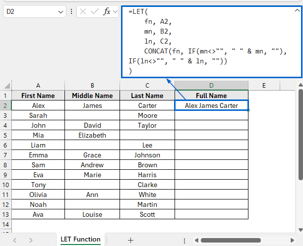
➧ fn, A2, part assigns the value from cell A2 into the fn variable.
➧ mn, B2, part assigns the value from cell B2 into the mn variable.
➧ ln, C2, part assigns the value from cell C2 into the ln variable.
➧ CONCAT(fn, IF(mn<>"", " " & mn, ""), IF(ln<>"", " " & ln, "")) combines the values stored in the variables fn, mn, and ln into a single text string. It adds a space before the middle name only if mn is not empty, and similarly adds a space before the last name only if ln is not empty.
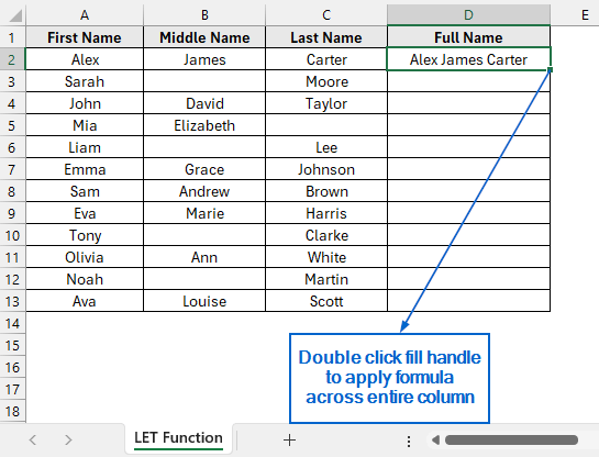
➤ Now, double-click the fill handle of cell D2 and apply the formula to the remaining cells in the column.
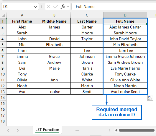
➤ Column D, containing the merged Full Name of the employee, should now be displayed.
Frequently Asked Questions
What Happens if I Have Empty Cells in My Dataset?
You might get unwanted extra spaces while merging cells if your dataset contains empty values. To avoid this, use functions like TEXTJOIN, CONCAT, or LET, which can handle empty cells more effectively.
Which Method Should I Use for Handling Large Datasets?
If you’re working with large datasets, the Power Query or LET function method is ideal, as both are optimized for performance and can handle high volumes of data more efficiently than traditional formulas.
Concluding Words
Knowing how to merge multiple columns in Excel is essential for organizing large datasets and managing information more efficiently. In this article, we have discussed six important methods of merging 3 columns in Excel, including using the TEXTJOIN Function, Ampersand (&) with IF Function, Power Query, CONCATENATE, CONCAT with IF and LET Functions. Feel free to try out each method and select one that best aligns with your needs.