
A workflow chart in Excel visually represents the sequence of steps in a process, making it easier to understand, analyze, and improve operations. With Excel’s built-in tools like Shapes, Connectors, and SmartArt, we can easily create a workflow chart to visualize the workflow.
Follow the steps below to create your very own workflow chart using Excel:
➤ Start by adjusting row height and column width to approximately 0.50 inches.
➤ Then, from the main menu, head to Insert >> Illustrations >> Shapes.
➤ Select and draw appropriate shapes to build your flowchart blocks.
➤ Next, connect the shapes by using arrows for directional flow.
➤ Finally, group and align the elements for a clean layout.
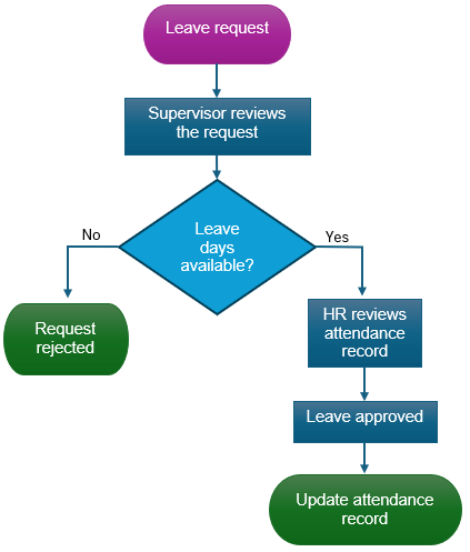
In this article, we will learn how to create a workflow chart in Excel by following five simple steps.
Steps to Creating a Workflow Chart in Excel
Creating a workflow chart in Excel is straightforward when you use the right tools. Follow the steps below to easily build a professional-looking workflow chart in Excel.
Step 1: Adjust the Cell Height and Width
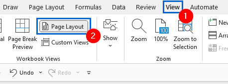
➤ Open the dataset and from the main menu, head to View >> Page Layout.
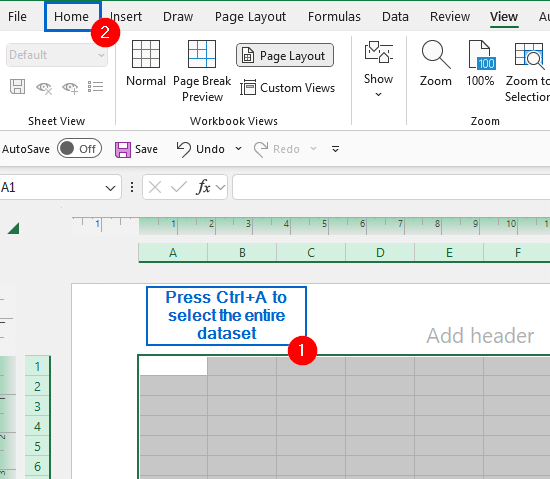
➤ Next, press Ctrl + A to select all cells in the dataset and head to the Home tab.
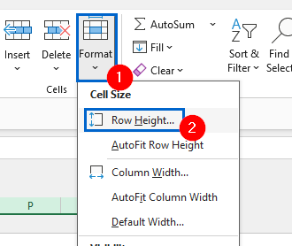
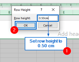
➤ From the Home tab, go to Format >> Row Height.
➤ In the Row Height dialogue box, type “0.50cm” to set the new height, then click OK.
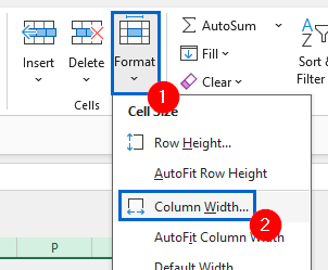
➤ Again from the Home tab, go to Format >> Column Width.
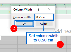
➤ Then, in the Column Width dialogue box, type “0.5cm” to set the new width and click OK.
Note:
Adjusting row and column heights to equal size ensures a uniform grid, making it easier to place shapes and arrows while maintaining consistent spacing between elements.
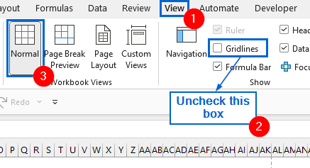
➤ Lastly, head to View, uncheck the Gridlines box and select Normal view.
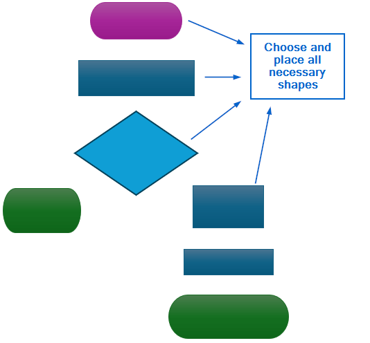
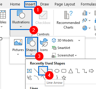
Step 2: Insert Flowchart Shapes
➤ To add flowchart shapes, go to the Insert >> Illustrations >> Shapes.
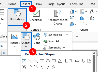
➤ From the Flowchart section, choose and place the necessary shapes based on your process.
Note:
You can also customize the appearance of your shapes by going to Shape Styles and selecting a preferred option from the Theme Styles gallery.
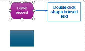
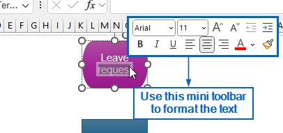
Step 3: Add Text Inside Shapes and Format Them
➤ Double-click on the shape to activate text editing and type your desired text.
➤ Use the mini toolbar to format text, adjust the font type, size, and alignment to match your preferred style.
➤ Next, resize the shape by clicking and dragging its corner or side handles.
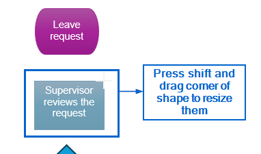
Note:
Press and hold the Shift key while dragging shapes to maintain their proportions.
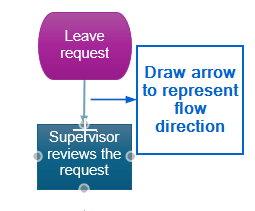
Step 4: Add Connector Arrows to Show Process Flow
➤ Head to the main menu and select Insert >> Illustrations >>Shapes >> Line Arrow.
➤ Draw arrows from one shape to another to represent the flow direction.
Note:
Hold down the Shift key while drawing arrows to ensure they remain perfectly straight and aligned with the flowchart shapes.
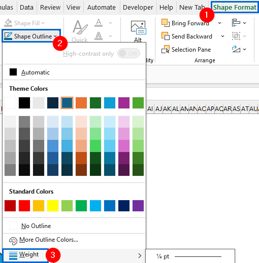
➤ Next, change the appearance and width of the arrow by heading to Shape Format >> Shape Outline >> Weight.
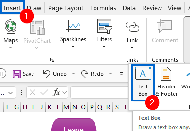
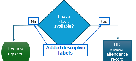
➤ Finally, add descriptive labels above the arrows by going to Insert >> Text Box and placing them near the connectors.
Step 5: Group Shapes for Easy Movement
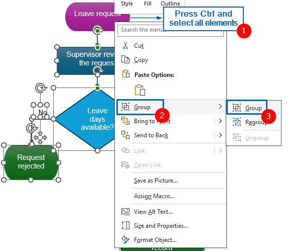
➤ Press and hold Ctrl , then select all the shapes and arrows.
➤ Next, right-click on any selected shape, and from the context menu, choose Group >> Group.
Note:
Grouping objects allows users to easily move, resize or format the whole workflow chart as a single unit.
Frequently Asked Questions
Can I Create a Workflow Chart in Excel Using SmartArt?
Yes, you can easily create a workflow chart in Excel using the SmartArt feature.
Head to the Insert tab from the main menu, click on SmartArt, and choose a layout that suits your workflow process. From there, you can customize the shapes, add text, and adjust colors to match your design needs.
How do I Properly Print the Workflow Chart From Excel?
To print the workflow chart without any extra space, select the entire chart area, then go to Page Layout >> Print Area >> Set Print Area. After that, navigate to File >> Print to preview and print the chart.
Can I Copy the Workflow Chart from Excel to PowerPoint or Word?
To copy the workflow chart into other applications, first select the grouped shapes and press Ctrl + C . Then, open Word or PowerPoint and press Ctrl + V . The chart will be pasted as an image or object that you can reposition or resize as needed.
Concluding Words
Knowing how to create a workflow chart in Excel is necessary for visualizing processes, improving clarity, and streamlining operations. In this article, we have discussed how to create a workflow chart in Excel using five simple steps. Feel free to practice all these steps to easily build your own customized workflow chart.