After creating a Pivot Table, you might need to add more data to your source sheet. Often, you will notice that your newly added data is not reflected in the Pivot Table. This problem often occurs when your PivotTable is not looking at the entire range of data. In this article, we will walk you through the most common reasons a PivotTable might not be picking up your data and show you how to fix it with different techniques.
To solve Pivot Table not picking up data, here is one simple solution by changing the data source.
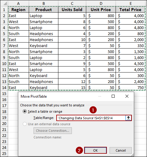
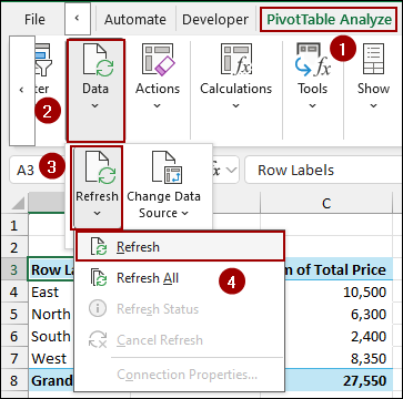
➤ After adding new data in the source sheet, go to PivotTable Analyze > Data > Change Data Source.
➤ In the Table/Range field, select the entire range with the newly added data.
➤Click OK, and you will see that your pivot table is picking all the data, including the newly added data, too.

Change the Data Source Range
One of the most common reasons a PivotTable does not update is that its data source range is fixed and doesn’t automatically expand when you add new rows. To solve this, you need to change the data source for the Pivot Table.
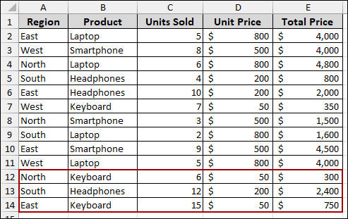
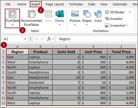
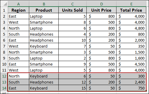
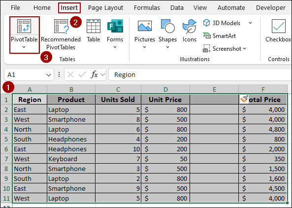
Imagine we have a sales dataset containing Region, Product, Units Sold, Unit Price, and Total Price.
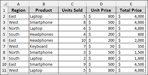
Now, we will create a Pivot Table with this sample data.
➤ Select the entire range and click Insert > PivotTable.
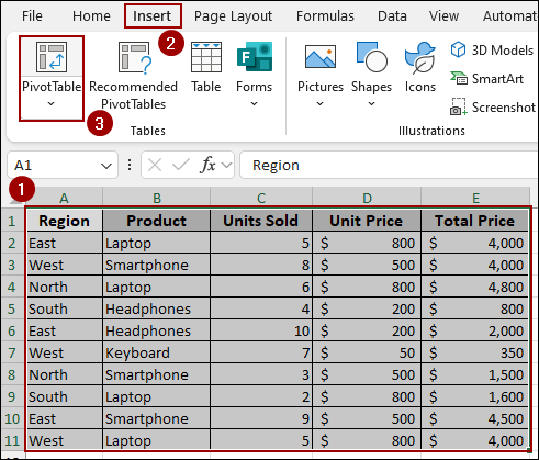
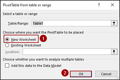
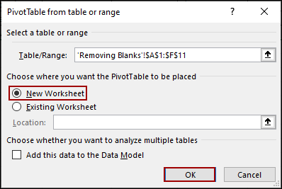
➤ Choose New Worksheet and hit OK.
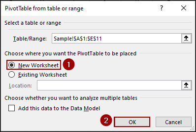
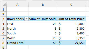
Thus, your Pivot Table will be created.
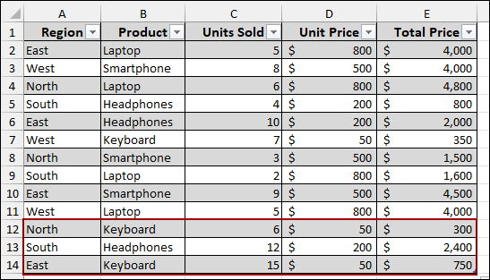
Now, let’s add some more sales data to the source sheet.
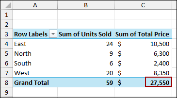
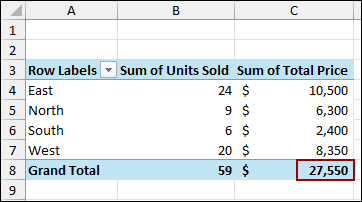
Coming back to the Pivot Table, we will see that the Pivot Table is not updated with the newly added data.
To fix this, we need to change the data source.
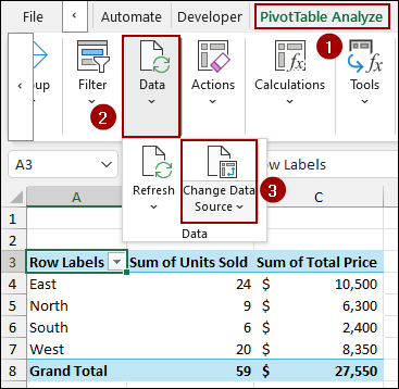
➤ Go to the PivotTable Analyze tab.
➤ In the Data group, click the dropdown menu for Data and select Change Data Source.
➤ In the Move PivotTable window, click the arrow in the Table/Range field. Now, select the entire updated range, from A1:E14.
➤ Click OK.
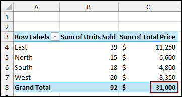
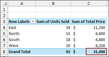
Finally, you will see that the PivotTable has been updated with the new data, and the Grand Total is now $31,000.
Convert Data to an Excel Table
The easiest way to prevent a PivotTable from failing to pick up new data is to convert your data range into an Excel table. An Excel table automatically expands to include any new rows or columns you add, so your PivotTable will always be up-to-date.
To convert your data to an Excel Table:
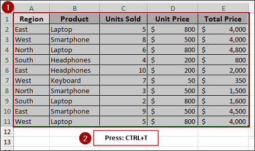
➤ Select your data range.
➤ Press Ctrl + T on your keyboard.
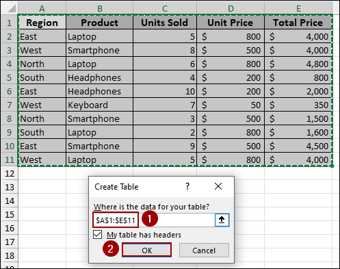
A Create Table dialog box will appear.
➤ Choose your data range and click OK.
Your data is now a formatted Excel Table.
Now, let’s create a PivotTable from this new table.
➤ Select your table.
➤ Go to the Insert tab and click PivotTable.
➤ Choose New Worksheet for your PivotTable and click OK.
Thus, the Pivot Table is created.
Now, let’s add some new data to the table. You will notice how the table automatically expands to include the new rows.
➤ Coming back to the Pivot Table sheet, go to the PivotTable Analyze tab and click Refresh in the Data group.
As a result, your PivotTable will now include the new data and update the totals.
Check for Hidden Data
Sometimes, a Pivot Table might not include data because it is filtered or hidden. When rows are hidden, the PivotTable will not count them unless you change your filter. To solve this issue, you need to remove the filter.
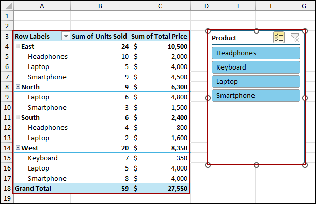
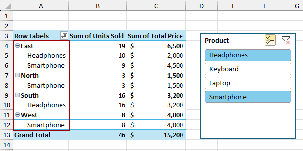
Here, we have created a Pivot Table following the steps from the previous method. We have a Slicer to filter the data for the Pivot Table.
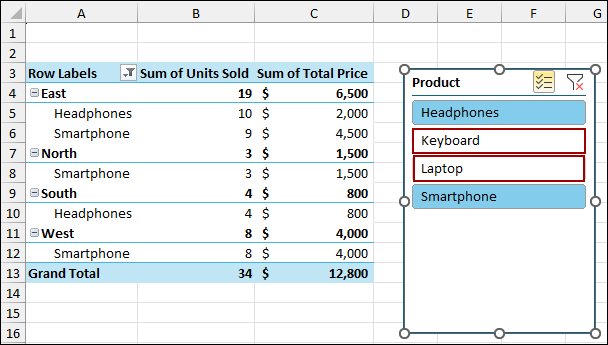
Now, let’s apply a filter using the Slicer. Here, we have deselected the Keyboard and Laptop using Slicer. Thus, the Pivot Table has removed all the data for the Keyboard and Laptop sales.
Coming back to the source sheet, let’s add some new data.
After adding the new data, you will see that the Pivot Table has not picked up the data as the filter is applied to the table.
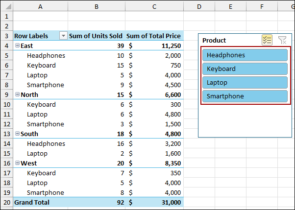
To solve this, choose all the products from the Slicer to show all the data or remove the Slicer. This way, the Pivot Table will pick up all the data.
Remove Blank Columns
A Pivot Table will not work correctly if there is a blank column in your source data. You just need to remove blank columns, and your Pivot Table will pick all the data.
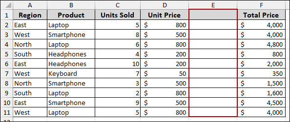
Suppose you have a dataset with a blank column.
Let’s create a Pivot Table with the blank column. For this,
➤ Select the range and click Insert > PivotTable.
➤ Choose New Worksheet and click OK.
Excel will give you the error “The PivotTable field name is not valid”.

To fix this, you must delete the blank column.
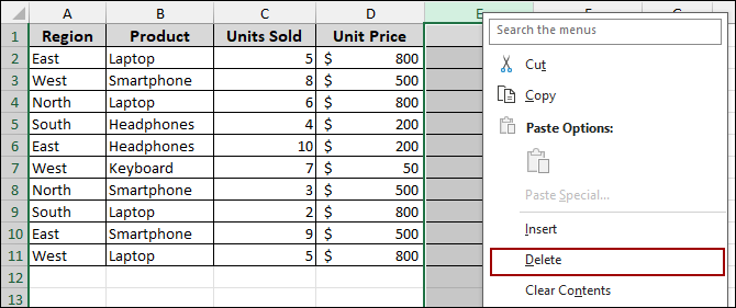
➤ Right-click on the blank column header (for example, column E).
➤ Select Delete from the context menu.
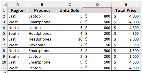
The blank column will be removed, and now if we create a Pivot Table, it will pick up data properly.
Ensure Headers in Source Data
Just like blank columns, missing headers in your source data will also cause a PivotTable to fail. If you want your Pivot Table to pick up data properly, every column in your dataset must have a unique header.
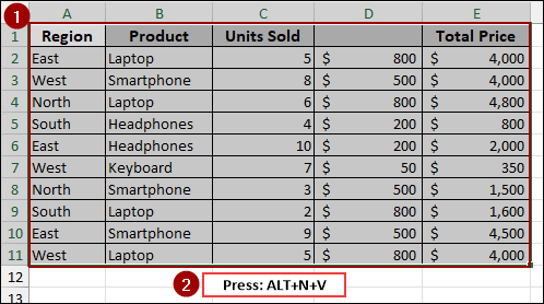
Imagine you have a dataset where one of the headers is blank, such as Column D.
➤ To create a Pivot Table, choose the data range and press Alt + N + V .
You will get the same error, “The PivotTable field name is not valid”.

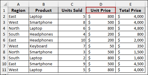
To solve this, simply add a header to the blank column. Now, select the data and create your Pivot Table. It will now work correctly, as all columns have a header.
Frequently Asked Questions
Why is the “Change Data Source” option greyed out?
This happens when your Pivot Table is based on a data model, external source, or Power Query connection. In such cases, you need to edit the query instead of manually changing the range.
My Pivot Table is not picking up numbers, only showing them as text. Why?
If numbers are stored as text values in the dataset, the Pivot Table won’t aggregate them properly. Convert them back to numbers using the VALUE function or by reformatting the cells.
I added calculated fields, but the results don’t update. What should I do?
Calculated fields rely on the Pivot Table cache. Refresh your Pivot Table or rebuild the calculated field if the formula references have changed.
Concluding Words
Above, we have explored all the reasons and solutions when you face a problem with your Pivot Table not picking up data. By understanding the common problems like fixed data ranges, hidden rows, or missing headers, you can quickly solve the problem. The best solution is to always format your data as an Excel table before creating a PivotTable. If you have any queries, don’t forget to let us know in the comments section below.