Collapsing the rows in a pivot table allows you to view the dataset more simply. Imagine you have a pivot table with a lot of data. It is hard to focus on a row when the pivot table is expanded. Collapsing the rows will help in understanding and analyzing the data better. In this article, we will learn how to collapse all rows in a pivot table in Excel. We will also learn some shortcuts so that you can do it as fast as possible to save your time.
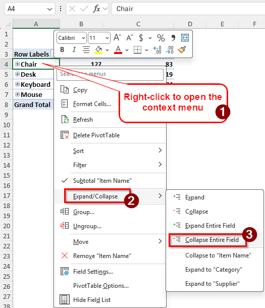
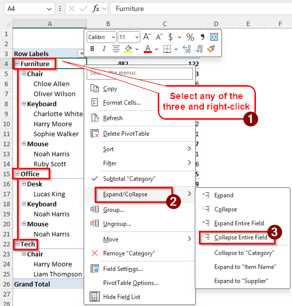
➤ Right-click on any of the field that belongs to the top rows of the pivot table.
➤ Select Expand/Collapse > Collapse Entire Field
In this article, we will learn five ways to collapse all rows in a pivot table. Each one has its place in the data analysis field, and you can choose which one you like. By the end of the article, you will know everything you can know about collapsing rows in a pivot table.
Using the Context Menu to Collapse All Rows in the Pivot Table
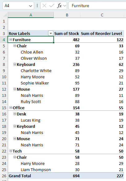
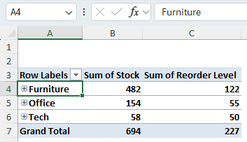
To make you understand all the methods in this article, we have picked a dataset with stock information. There are item names, the categories of those items, the stock level, the reorder level, and the supplier of the items. We will collapse the rows in the pivot table so that the table gets smaller and we get the data according to the top row.
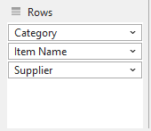
➤ First, take a look at the rows section. There are three fields in this section: Category, Item Name, and Supplier.
➤ If we collapse the Category field, all of the rows under those will be collapsed as well. They will technically still be expanded, but as the top row is collapsed, the rest won’t show.
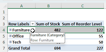
➤ Right-click on a cell in the pivot table that belongs in the Category field. In this pivot table, those cells are A4, A15, and A22.
➤ Go to Expand/Collapse > Collapse Entire Field. This will collapse the whole Category field.
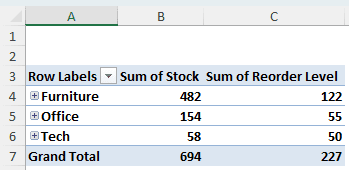
➤ Now all of the rows in the pivot table are collapsed.
Making Use of the Ribbon to Collapse All Rows in the Pivot Table
The ribbon in Microsoft Excel has a lot of options to manipulate your pivot table. We can make use of it to collapse the rows as well. Let’s learn how to do it:
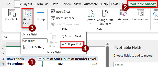
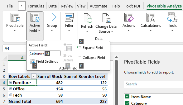
➤ Go to one of the cells from the top of the rows as suggested in the previous method. We are going to the A4 cell for now.
➤ Head to the PivotTable Analyze tab of the Ribbon. Find the Active Field section in the tab.
➤ Click on Collapse Field to collapse all rows.
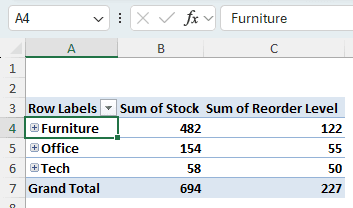
➤ Check the table to see the results.
Utilizing Keyboard Shortcuts to Collapse the Rows in the Pivot Table
The ribbon method can easily be employed using keyboard shortcuts in Microsoft Excel. Follow the steps below to learn to do it:
➤ Like the methods mentioned before, choose a cell from the top of the Rows section. We are going for the A4 cell again.
➤ Press the keys serially to collapse the rows. Do not press them at once; you must press them serially, one by one.
Alt > J > T > P
Collapsing All Rows of the Pivot Table with Keyboard and Mouse
Probably the easiest method to collapse the rows is using the keyboard and mouse. Just follow the steps below to do it:
➤ Click on the cell of the field that you want to collapse. We want to collapse all of the fields, so we want to go to the first field of the Rows section. It’s going to be the A4 cell here.
➤ Keep the mouse cursor in that cell, and press Shift . When pressing Shift , move the scroll wheel down. All of the rows will be collapsed.
Applying VBA Code to Collapse All Rows in the Pivot Table
If you aren’t satisfied with manual methods, we can automate it using VBA code. VBA in Microsoft Excel allows automating a lot of worksheet functions, and we can use it to collapse all the rows we want. If you want to learn advanced Microsoft Excel, you should go this route.
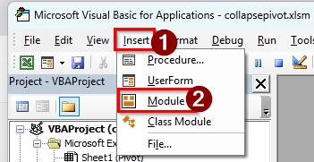
➤ Press Alt + F11 to open the “Microsoft Visual Basic for Applications” window.
➤ From the menu bar at the top, go to Insert > Module.
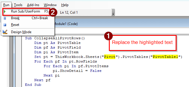
➤ A new window will open inside the existing window. You need to write the following code in that window:
Sub CollapseAllPivotRows()
Dim pt As PivotTable
Dim pf As PivotField
Dim pi As PivotItem
Set pt = ThisWorkbook.Sheets("Pivot").PivotTables("PivotTable1")
For Each pf In pt.RowFields
For Each pi In pf.PivotItems
pi.ShowDetail = False
Next pi
Next pf
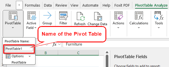
End Sub➤ Replace “Pivot” with the name of the worksheet, and “PivotTable1” with the name of the pivot table. You can get the name of the pivot table from the PivotTable section of the PivotTable Analyze tab.
➤ Go to the code window and go to Run > Run Sub/UserForm from the top bar.
➤ Go back to the worksheet to see the result. The best thing about this method is that it collapses the fields under the top row as well, so when you expand the first one, you see that the other ones are still collapsed.
Frequently Asked Questions
How to collapse multiple rows in Excel?
First, select which rows you want to collapse. Then, go to the Data tab, and go to the Outline section. From there, find the Group icon and click on it. In the new window, select Rows and click OK. On the left of the table, you will find some minus (–) signs now. Click on those signs to collapse the rows. You can collapse as many rows as you want using this method.
How to flatten PivotTable rows?
Select any of the cells of the pivot table, and go to the Design tab. Find the Layout section on the left, and locate the Report Layout icon. Click on it to open, and select “Show in Tabular Form” to flatten the rows of the pivot table.
How to show PivotTable fields?
Select a cell in the pivot table; any of the cells will work. Right-click on the cell, and select Show Field List. Now the PivotTable Fields panel will show up.
How to hide totals in a PivotTable?
First, make sure that the pivot table is selected. In the ribbon at the top, go to the Design tab. From the Layout section of the tab, go to either the Subtotals or the Grand Totals button. In the Subtotals icon, select Do Not Show Subtotals. In the Grand Totals icon, select Off for Rows and Columns from the drop-down menu.
How to shrink multiple rows in Excel?
Select the rows you want to shrink in Microsoft Excel. On the left, where the row numbers are indicated, right-click and select Row Height. Change the value to a lower number and press OK to shrink the rows.
Wrapping Up
In this article, we have learned five ways to collapse all rows in a pivot table. If you have any other methods to do this, share them with us below. Download the Excel file we used in this article to practice the method. The VBA code we used is also there so that you can see the code in action. Thanks for reading, see you next time.