While working with datasets in Excel, it is often required to return values based on multiple criteria. By combining COUNTIF with INDEX and MATCH functions, we can effortlessly perform this operation.
Follow the steps below to look up a value in your dataset based on multiple criteria using the INDEX, MATCH and COUNTIF functions:
➤ In your dataset, navigate to the cell where you want to return the multi-criteria lookup value and paste the following formula:
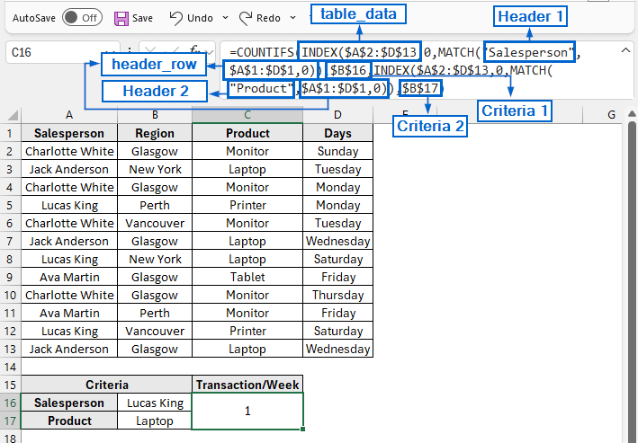
=COUNTIFS(INDEX(table_data, 0, MATCH(header1, header_row, 0)), criteria1, INDEX(table_data, 0, MATCH(header2, header_row, 0)), criteria2)
➤ Replace header_row with the range that contains your column headers.
➤ Replace table_data with the range of actual datasets from which the formula will pull information.
➤ Replace header1 with the text of the first column header you want to filter by.
➤ Replace criteria1 with the cell reference containing the first lookup value.
➤ Replace header2 with the text of the second column header you want to filter by.
➤ Replace criteria2 with the cell reference containing the second lookup value.
In this article, we will learn how to use INDEX and MATCH functions along with COUNTIF to perform lookups within a dataset based on two, three and four criteria.
Combine INDEX-MATCH with COUNTIF for Two Criteria Lookup
In the sample dataset, we have a worksheet called “Product Details” containing information about Salesperson, Region, Product and Days of the week (Sunday through Saturday) on which each product was sold.
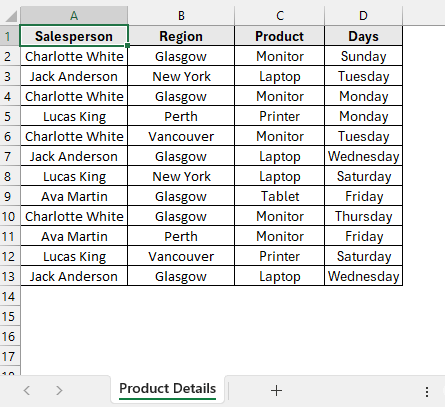
By combining the INDEX and MATCH functions with COUNTIF, we will determine how many transactions took place in a week based on the criteria entered in the Salesperson and Product fields. The updated dataset will be stored in a separate “Two Criteria” worksheet.
INDEX, MATCH, and COUNTIF are powerful Excel functions that allow users to search, retrieve, and count values within a dataset based on defined criteria. By combining these three functions, we can return a specific value from a dataset while evaluating multiple criteria at once.
Steps:
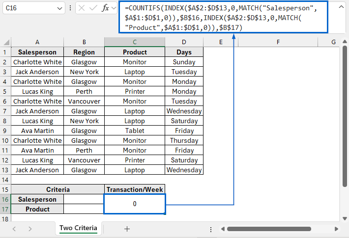
➤ Open the Two Criteria worksheet and in cell C16 paste the following formula:
=COUNTIFS(INDEX($A$2:$D$13,0,MATCH("Salesperson",$A$1:$D$1,0)),$B$16,INDEX($A$2:$D$13,0,MATCH("Product",$A$1:$D$1,0)),$B$17)
➧ MATCH("Salesperson",$A$1:$D$1,0) part finds a column number where the header "Salesperson" is located within $A$1:$D$ header row.
➧ INDEX($A$2:$D$13,0, … ) uses that column number to return the entire "Salesperson" column from the range $A$2:$D$13.
➧ INDEX(...), $B$16 checks the "Salesperson" column against the value entered in cell B16.
➧ MATCH("Product",$A$1:$D$1,0) finds the column number where the "Product" header is located.
➧ INDEX($A$2:$D$13,0, … ) returns the “Product” column from the data range.
➧ INDEX(...), $B$17 part checks the “Product” column against the value entered in cell B17.
➧ COUNTIFS( … ) finally counts how many rows in the dataset (A2:D13) satisfy both conditions.
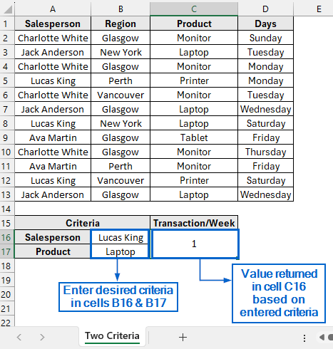
➤ Next, enter the criteria that you want to search for in cells B16 and B17.
➤ Cell C16 should now return a value based on the entered criteria.
Combine INDEX-MATCH with COUNTIF for Three Criteria Lookup
Building on the previous method, we can extend the use of INDEX, MATCH, and COUNTIF functions to perform a lookup based on three criteria as well.
Using the same dataset, we will now apply all three functions together to determine the number of transactions that occurred during the week based on the three criteria entered in cells B16, B17, and B18, respectively. The updated dataset will be stored in a separate worksheet called “Three Criteria”.
Steps:
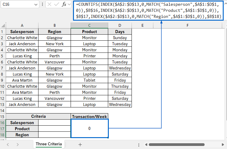
➤ Open the Three Criteria worksheet and in cell C16 paste the following formula:
=COUNTIFS(INDEX($A$2:$D$13,0,MATCH("Salesperson",$A$1:$D$1,0)),$B$16,INDEX($A$2:$D$13,0,MATCH("Product",$A$1:$D$1,0)),$B$17,INDEX($A$2:$D$13,0,MATCH("Region",$A$1:$D$1,0)),$B$18)
➧ MATCH("Region",$A$1:$D$1,0) part finds the column number where the "Region" header appears in the header row $A$1:$D$1.
➧ INDEX($A$2:$D$13,0, … ) uses that column number to return the entire “Region” column from the dataset.
➧ INDEX(...), $B$18 part compares the “Region” column against the value in cell B18.
The rest of the formula works the same way as the first method with two criteria.
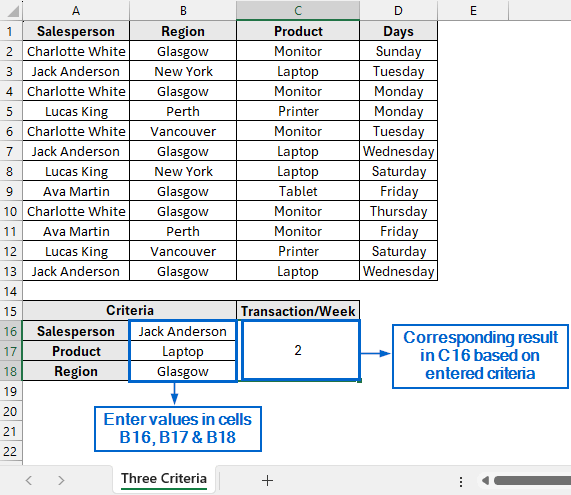
➤ Enter your desired criteria into cells B16, B17 and B18.
➤ The corresponding result for these criteria will automatically appear in cell C16.
Combine INDEX-MATCH with COUNTIF for Four Criteria Lookup
Working again with the same dataset, we will now use INDEX, MATCH, and COUNTIF functions together to calculate the number of transactions that occurred during the week, this time based on the four criteria entered in cells B16, B17, B18, and B19. We will display the modified dataset in a separate “Four Criteria” worksheet.
Steps:
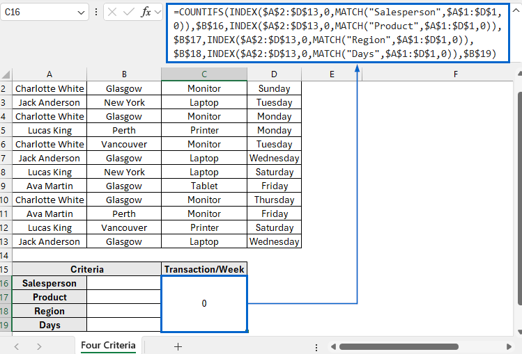
➤ Open the Four Criteria worksheet and in cell C16 paste the following formula:
=COUNTIFS(INDEX($A$2:$D$13,0,MATCH("Salesperson",$A$1:$D$1,0)),$B$16,INDEX($A$2:$D$13,0,MATCH("Product",$A$1:$D$1,0)),$B$17,INDEX($A$2:$D$13,0,MATCH("Region",$A$1:$D$1,0)),$B$18,INDEX($A$2:$D$13,0,MATCH("Days",$A$1:$D$1,0)),$B$19)
➧ MATCH("Days",$A$1:$D$1,0) part finds the column number where the "Days" header is located in the header row $A$1:$D$1.
➧ INDEX($A$2:$D$13,0, … ) uses that column number to return the “Days” column from the dataset.
➧ INDEX(...), $B$19 compares the “Days” column against the value entered in cell B19.
Aside from the new additional criteria, the formula operates the same way as in the previous two methods.
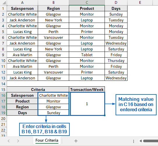
➤ Input the criteria you want to search for in cells B16, B17, B18 and B19.
➤ The result matching these inputs will be displayed in cell C16.
Frequently Asked Questions
Can I Use INDEX, MATCH, and COUNTIF Functions to Perform Lookup with More Than Four Criteria?
Yes, you can do so by extending the formula and adding more conditions inside the COUNTIF function. For each additional criterion, pair the lookup value with its corresponding column using INDEX and MATCH functions.
Is this Method Suitable for Dealing with Large Datasets?
COUNTIF with INDEX–MATCH is generally efficient for handling large datasets because it avoids using array formulas. However, when working with very large ranges, you can improve performance by converting your dataset into an Excel table.
Wrapping Up
Knowing how to use the INDEX and MATCH functions with COUNTIF for multi-criteria lookup is essential for efficiently analyzing data and simplifying complex searches. In this article, we have discussed how you can use the INDEX, MATCH, and COUNTIF functions to perform lookups based on two, three, and four criteria. Feel free to practice with the dataset and choose the method that best fits your lookup criteria.