How to Show Column Numbers Instead of Letters in Excel

Working with large spreadsheets, counting columns, or following formulas gets a little tricky. Excel labels columns with letters by default, but sometimes it’s easier to follow along when columns are numbered.

In this guide, we’ll show you a couple of simple ways to switch column headers from letters to numbers or add a quick number reference to your sheet. This will help you stay on track, especially when working with wide tables.

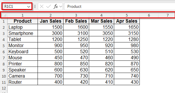
This is the only built-in way to properly change Excel’s column headers from letters to numbers across the entire grid. After turning on R1C1 reference style, column headers change from A, B, C to 1, 2, 3.  It also changes how formulas are displayed from =A1+B1 to =RC+RC[-1]. This is helpful when you’re working with large spreadsheets, scripting with VBA, or using logic-based formulas that rely on row and column positions.

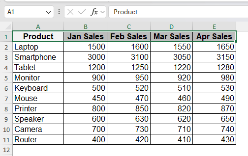
We’ll use a simple dataset of Product Inventory with monthly stock updates and reorder levels to show how to apply different methods more efficiently and accurately.

Steps:

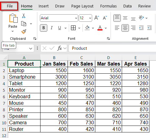
➤ Click on File from the top left of Excel.

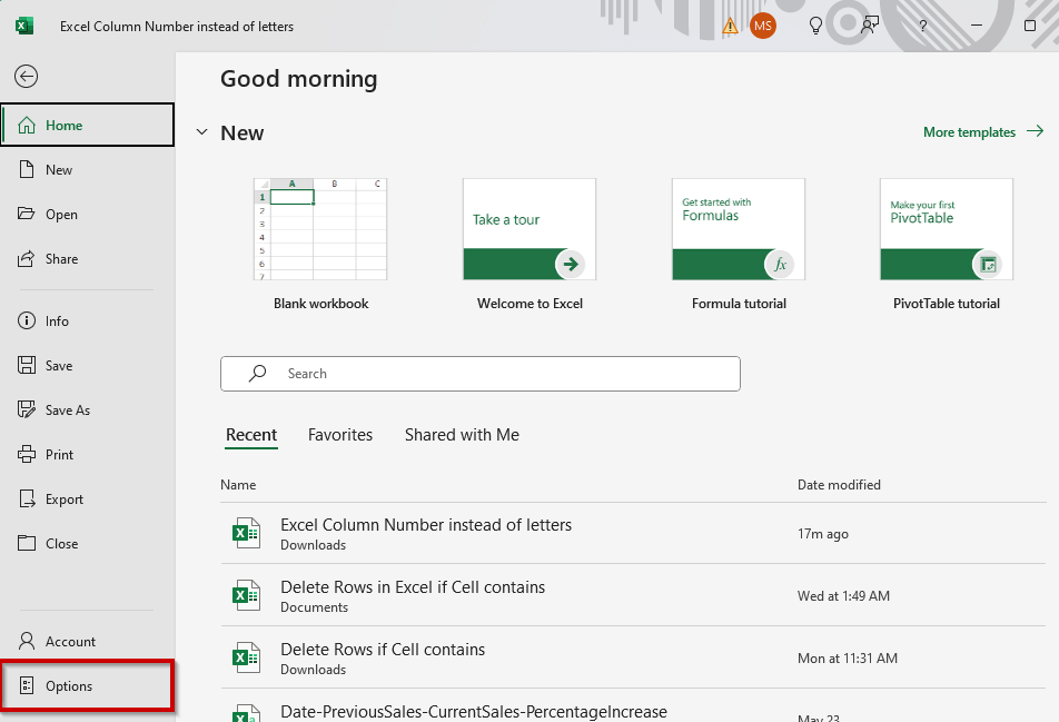
➤ Choose Options at the bottom of the menu.

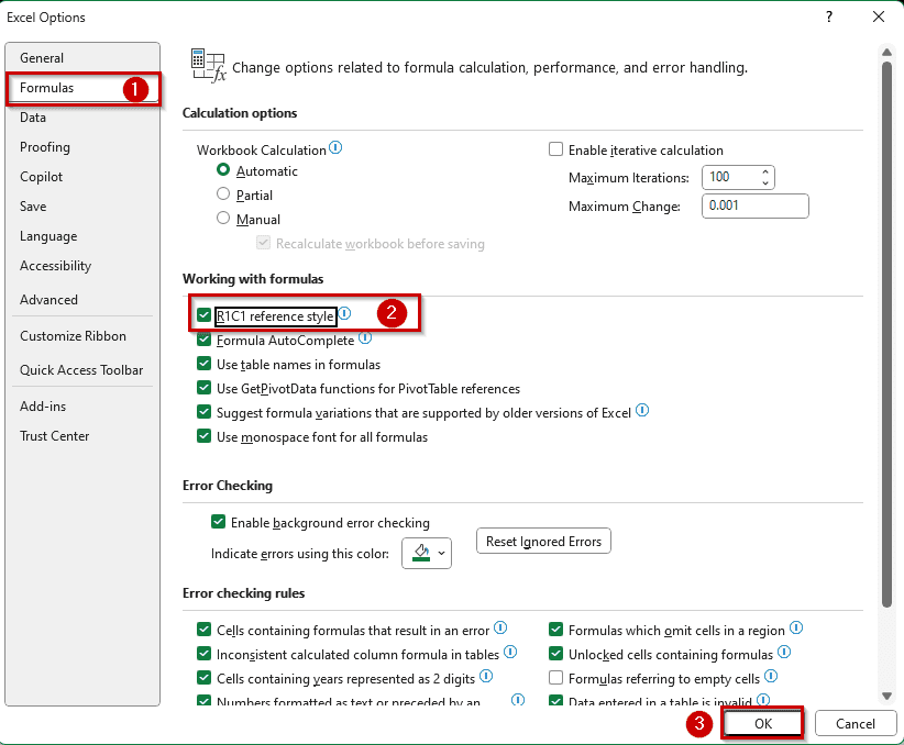
➤ In the Excel Options window, go to formulas.
➤ Under “Working with formulas”, tick the checkbox that says R1C1. Click OK.

 ➤ Here is the result with column numbers instead of letters.

If you want to see column numbers without changing how Excel works behind the scenes, adding a helper row is the easiest way. This method doesn’t replace the default A, B, C column headers, but gives you a visible number reference just below them. Use this method when you’re working with wide tables or when you want to share the sheet with someone unfamiliar with the structure.

This goes well when planning reports, printing sheets, or building formulas based on column positions. This method also works well in print layouts, where Excel letter headers are not shown by default. Having a numeric row at the top helps keep things clear on paper. It doesn’t affect any formulas, sorting, or filters; it’s just a visual guide. Unlike R1C1, it doesn’t change Excel’s behaviour or formula language. It’s quick to set up., and even quicker to remove if needed.

Steps:

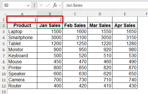
➤ Insert a new row at the top of your dataset.
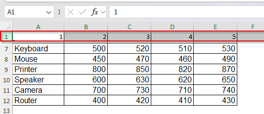
➤ In row 1, type 1 in A1, 2 in B1.

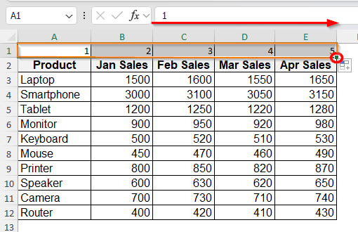
➤ Select both the cells and drag the fill handle to fill in numbers.

➤ Now select & freeze this row using View > Freeze Panes > Freeze Top Row to keep the helper row visible as you scroll down.

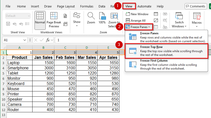
➤ Scroll up, and row 1 will stay frozen as it acts as a reference line for the column numbers.

When you switch to R1C1 Reference Style, Excel changes both header labels and formula format to numbers, giving you a clean, coordinate-style layout.

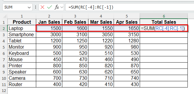
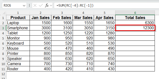
Let’s say your monthly sales sheet is in R1C1 mode. If you want Column F to show the sum of Jan-Mar for each product, you’ll write this formula in F2:

Here, R refers to the same row. C[-4] and C[-1] refer to four columns and one column left from F2.

Every row uses exactly the same formula, with no adjustments to cell letters. That consistency is especially helpful in large data tables, ensuring your sheet stays clean and consistent.

You’ll see how R1C1 simplifies formula replication, keeping your sheet neat. And since Excel records macros with R1C1 cell reference style, it aligns perfectly with VBA, no need to convert formulas mid-code.

Steps:

➤ Write the formula in cell F2, numbered as column 6.

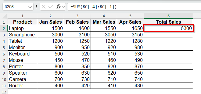
 ➤ Press Enter to see the result.

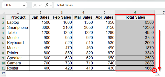
➤ Write the same formula in the next cell, F3.

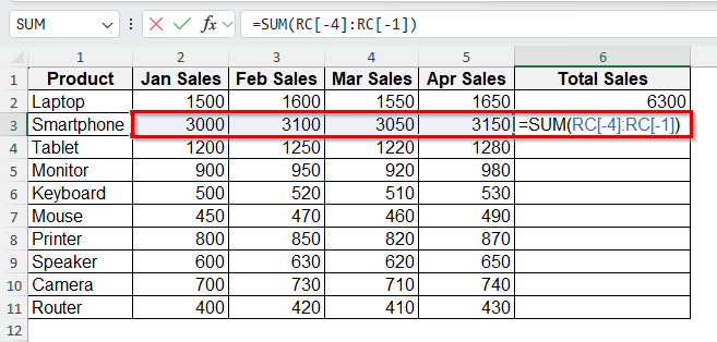
 ➤ The same formula will show the sum for sales of January-April.

➤ Drag the fill handle to get results for other rows.

Frequently Asked Questions

Why do my formulas look strange after enabling R1C1?

That’s expected, Excel rewrites formulas in this mode. RC means current cell, RC[-1] means the cell to the left, and so on.

Does R1C1 affect others using my file?

No. It’s only a display setting for your Excel app. The file itself doesn’t change.

Is there a shortcut to toggle R1C1 mode?

Not a keyboard shortcut, but it takes just a few clicks via File > Options > Formulas.

Can I use these tricks in Google Sheets?

No, you can’t. Google Sheets doesn’t support R1C1 mode.

Wrapping Up

Changing column letters to numbers in Excel is smoother than you think, especially in bigger spreadsheets. If you want a quick way to update the actual column headers, switching to R1C1 reference style is the simplest option. For those who just need a reference without changing settings, adding a helper row with numbers works just fine. Both ways help you stay more organised and make it easier to follow along with your data. Give it a try and let us know which one feels right for you.