If you want to reverse the order of data in a row or rearrange your dataset from right to left instead of left to right, Excel has several easy ways to flip data horizontally. Whether you’re working with timelines, ranking data, or just want to mirror cell order for comparison, flipping data horizontally is used for tasks like reversing a timeline, rearranging survey answers, or mirroring any set of data without manual rearrangement. The solution ranges from using formulas, sorting tricks, or even automation through VBA.
This guide walks you through different approaches to flip a single row of data horizontally, helping you reorganize your spreadsheet layout in a dynamic and efficient way. It also makes your spreadsheets more flexible and customized.
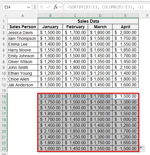
Steps to flip data horizontally by combining SORTBY and COLUMN functions:
➤ Select your desired data range, from B3 to E3.
➤ Use the formula: =SORTBY(B2:E2, COLUMN(B2:E2), -1)
➤ This formula flips the data from left to right of the range B2 to E2, adjusting as the original data changes.
➤ And here is the final result after filling in the formula for all other rows..

Flip Data Using Sort with a Helper Row
This is one of the most straightforward ways to flip data without using any formulas. When you just need to reverse the order of data across columns, this method does the job effectively.
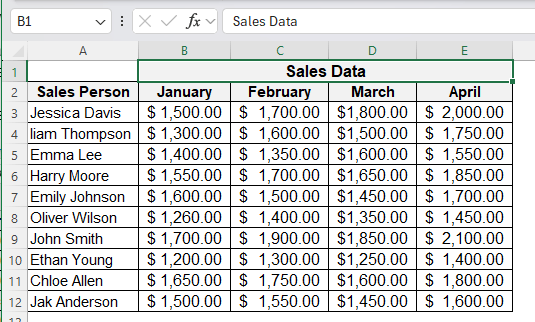
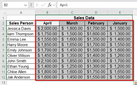
Here we will use a simple dataset containing months from January to April.
Steps:
➤ Insert a new row below your dataset.
➤ In this helper row, type sequential numbers starting from 1.
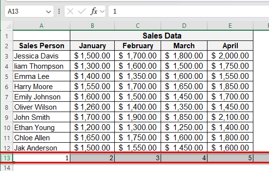
➤ Select both your data row and helper row.
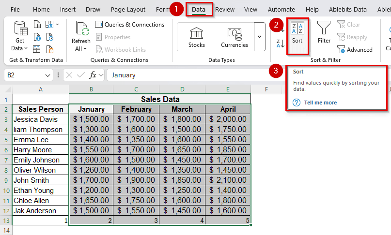
➤ Go to the Data tab and click Sort.
➤ Click on Options and choose Sort left to right.
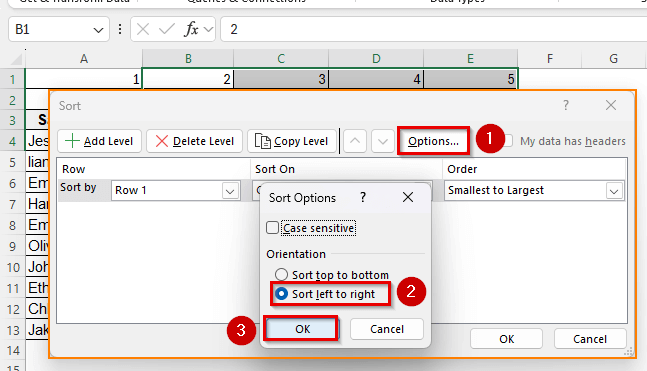
Note:
Make sure you select ‘My data has headers’.
➤ Under the Row dropdown, select your helper row, and set the order to Largest to smallest.
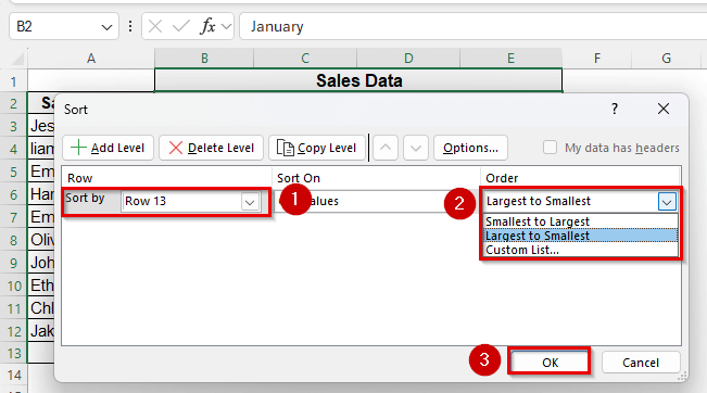
➤ Click OK, and your data will be flipped horizontally.
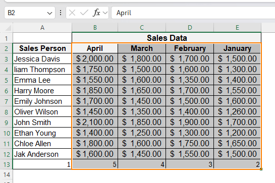
➤ Delete the helper row after sorting if you wish to keep the sheet clean.
Flip Data Horizontally Using Formulas (SORTBY)
For a dynamic approach where you want data to flip automatically with changes, Excel formulas can help. There are options for both newer and older Excel versions.
These formula-based methods work well when you want the flipped data to be updated automatically whenever you update the original dataset.
Steps for SORTBY(Excel 365 and Newer):
➤ Select your desired data range, from B3 to E3.
➤ Use the formula:
=SORTBY(B2:E2, COLUMN(B2:E2), -1)
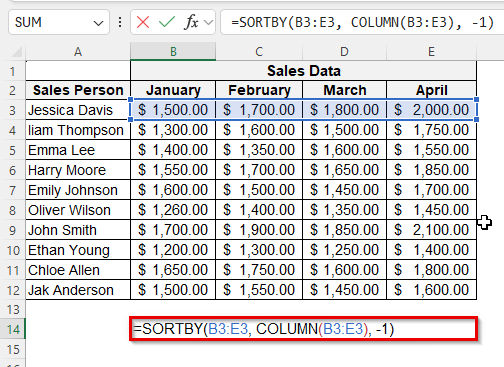
➤ This formula flips the data from left to right of the range B2 to E2, adjusting as the original data changes.
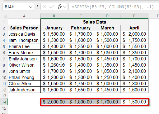
➤ And here is the final result after filling down the formula for all other rows.
Flip Data Horizontally Using VBA Macro
In order to flip data or to automate the process, use a simple VBA code, this method allows you to flip entire rows with just one click.
This VBA method is ideal when you have recurring tasks or large datasets where manual sorting or formulas become inconvenient. This saves time and effort, adding flexibility and speed.
Steps:
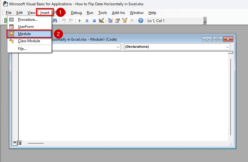
➤ Press Alt + F11 to open the VBA editor.
➤ Click Insert > Module.
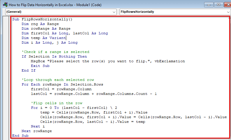
➤ Paste the following code:
Sub FlipRowsHorizontally()
    Dim rng As Range
    Dim rowRange As Range
    Dim firstCol As Long, lastCol As Long
    Dim temp As Variant
    Dim i As Long, j As Long
    'Check if a range is selected
    If Selection Is Nothing Then
        MsgBox "Please select the row(s) you want to flip.", vbExclamation
        Exit Sub
    End If
    'Loop through each selected row
    For Each rowRange In Selection.Rows
        firstCol = rowRange.Column
        lastCol = rowRange.Column + rowRange.Columns.Count - 1
        'Flip cells in the row
        For i = 0 To (lastCol - firstCol) \ 2
            temp = Cells(rowRange.Row, firstCol + i).Value
            Cells(rowRange.Row, firstCol + i).Value = Cells(rowRange.Row, lastCol - i).Value
            Cells(rowRange.Row, lastCol - i).Value = temp
        Next i
    Next rowRange
End Sub
➤ Save, close the editor, and go back to Excel.
➤ Press Alt + F8 , run FlipDataHorizontally after selecting the range, B3 to E12.
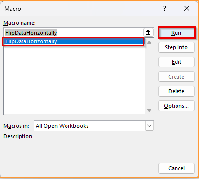
➤ This is the result that appears.
Flip Data Horizontally Using Add-ins
If you frequently need to manipulate data in Excel, third-party add-ins like Ablebits offer dedicated tools to flip data horizontally in a few clicks.
This method is suitable for advanced users who work with bulk datasets and want a ready-to-use solution without manual formulas or scripts.
Steps:
➤ Select your data range from B2 to E2.
➤ Go to the Ablebits Data Tab > Transform > Flip Horizontally.
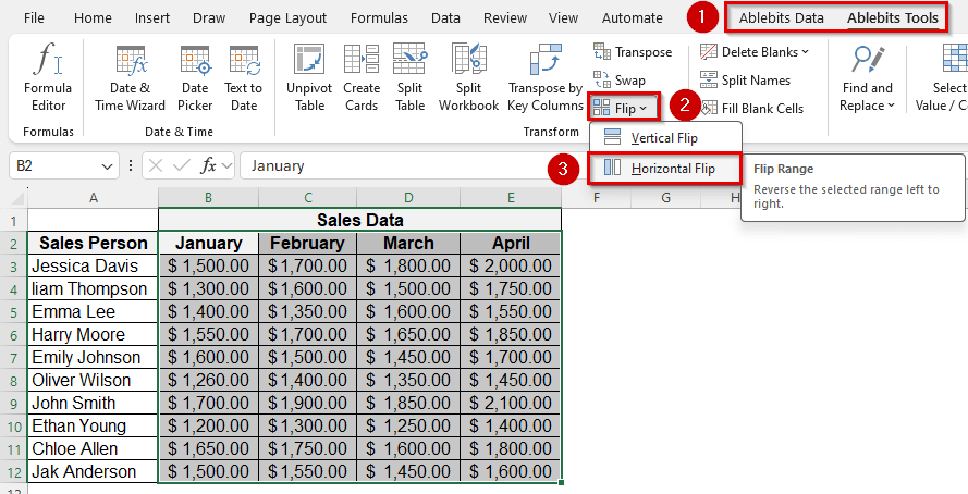
➤ Choose ‘paste values only’ > Flip.

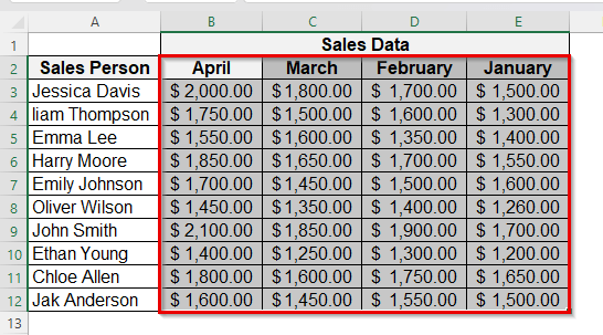
➤ Here is your result.
Frequently Asked Questions
Can I reverse column data using the same methods?
Yes, just transpose the columns into rows, flip horizontally, and transpose back.
Does the VBA method preserve cell formatting?
Yes, the VBA macro retains both formulas and formats while flipping the data.
Are these methods applicable to multiple rows?
Yes, you can select multiple rows and apply all methods except for the formula-based methods, which may need adjustments.
What’s the quickest way without formulas ot VBA?
Using the helper row with sorting is the fastest manual method without needing any scripts or formulas.
Wrapping Up
Flipping data horizontally in Excel is an easy process. Whether you prefer quick sort trick, dynamic formulas, or a one-click VBA solution, you can easily reverse the order of your row data. Use of the add-in, Ablebits tool, is even better for such work. Explore these methods to suit your workflow, whether for simple fixes or large data manipulations. Let us know which one fits your work the best.