In Excel, you often require the sum of ranges of cells based on some criteria. Usually, you can do this with SUMIFS for a single sum range. However, to do the same thing for multiple columns, you might need to think outside the box. It is often necessary when working on quarterly product summaries, academic scoring across tests, or production totals on multiple shipments. Above all, the best part is that you still have a wide range of tools in Excel to sum multiple columns with SUMIFS.
To sum ranges of multiple columns with SUMIFS, go step-by-step following this method –
➤ Open the worksheet and identify the columns you need to sum and your criteria.
➤ Select another cell where you want your desired output to show.
➤ The syntax of the SUMIF formula is – =SUMIF(range, criteria, [sum_range]),
where the first range is the number of cells that need to be summed, the criteria is the condition, and the sum_range is the range of columns added together.
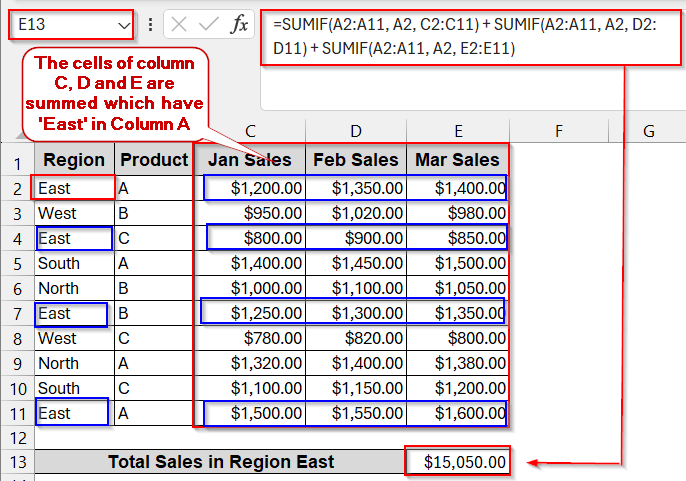
➤ For multiple columns, you can use the formula below –
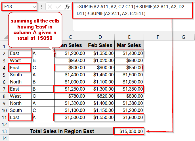
=SUMIF(A2:A11, A2, C2:C11) + SUMIF(A2:A11, A2, D2:D11) + SUMIF(A2:A11, A2, E2:E11)
Here, the A2:A11 is the first column range that determines the range, and C2:C11, D2:D11, and E2:E11 are the columns that need to be summed. A2 is the criterion or the condition based on which the sum is done.
➤ Press Enter. If needed, give it a proper header.
In this article, we will explore every practical method you will use while summing values from multiple columns based on specific criteria. Starting from the basic SUMIF formula and SUMPRODUCT, we moved to modern BYCOL+LAMBDA and OFFSET/INDEX array techniques. Lastly, we have covered it all with the non-formula approach of Power Query and VBA. Stay tuned with us through the whole process as we guide you to the best insights of each method.
Combine Multiple SUMIFS for a Multi-Column Total
As we know, the SUMIF formula is by default on a single column. But if your data spans multiple columns, you can still use the SUMIF individually for each column. And late sum them up. It is the easiest and beginner-friendly approach and can be easily done manually, adding or using the SUM formula.
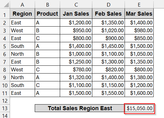
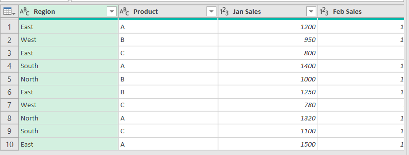
The dataset below will be used to illustrate the following methods.
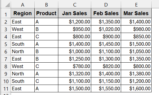
We will sum the sales values from January to March from the region ‘East’.
Steps:
➤ Open the dataset and choose the columns that you need to sum and the condition.
➤ Select the cell to show the result.
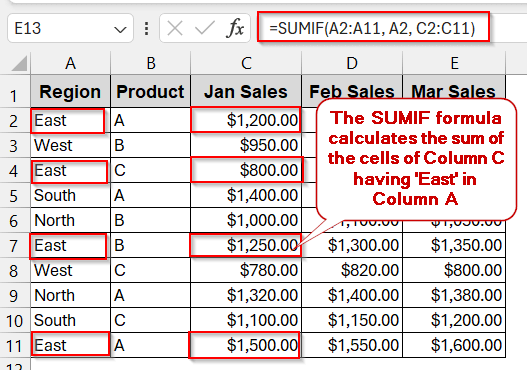
➤ Use the SUMIF formula for the column in this format-
=SUMIF(A2:A11, A2, C2:C11)
Here A2:A11 is the range, A2 holds the condition (or the text by which they are filtered), and C2:C11 is the column to be summed.
➤ for multiple columns, you add a SUMIFS formula for each one –
=SUMIF(A2:A11, A2, C2:C11) + SUMIF(A2:A11, A2, D2:D11) + SUMIF(A2:A11, A2, E2:E11)
Here, C, D, and E are the columns that need to be added for the sales, and A2 is the cell containing the region ‘East’ as a condition.
➤ Press Enter to view the result in the cell.
➤ Give an appropriate header for more readability.
Notes:
All the ranges must match in size to make this formula work.
Apply SUMIFS to Each Column Using BYCOL and LAMBDA Functions
For users of Excel 365, a better approach to use SUMIFS is to pair it up with BYCOL and LAMBDA. It has a cleaner formula structure and is also more readable without offset adjustments. For multiple column manipulation, this combination of formulas gives more accurate results with fewer hassles.
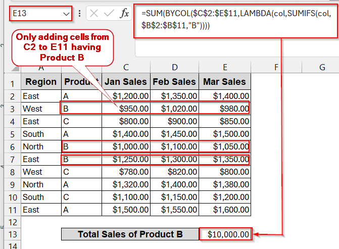
In this method, we will sum all the sales from January to March of Product B.
Steps:
➤ Open the Excel document and identify the columns and conditions you require.
➤ Select the cell to display the output of the formula.
➤ In the cell, write the formula of SUMIF with BYCOL+LAMBDA–
=SUM(BYCOL($C$2:$E$11, LAMBDA(col, SUMIFS(col, $B$2:$B$11, "B"))))
Here C2:E11 is the Jan to March sales and B2:B11 is the column of the Products. The SUMIFS(col, $B$2:$B$11, “B”) part ensures that the rows of column B having the product ‘B’ are added only.
➤ Press Enter to get the result in the cell.
➤ Give an appropriate header for proper definition.
Notes:
➨ BYCOL is only available in Excel 365; older versions will give no result for this formula.
➨ You can add more criteria by adding an extra criterion and a range inside the SUMIF formula.
Sum Non-Adjacent Columns with SUMIFS and OFFSET Using Array Constants
If you want more control over your SUMIFS and get advanced results with them, OFFSET can be very helpful. As it enables you to give array constants, the flexibility you get is much higher than the previous ones. But that’s not yet the best part. Combining OFFSET with the SUMIF formulas also enables you to sum the columns that are not beside each other.
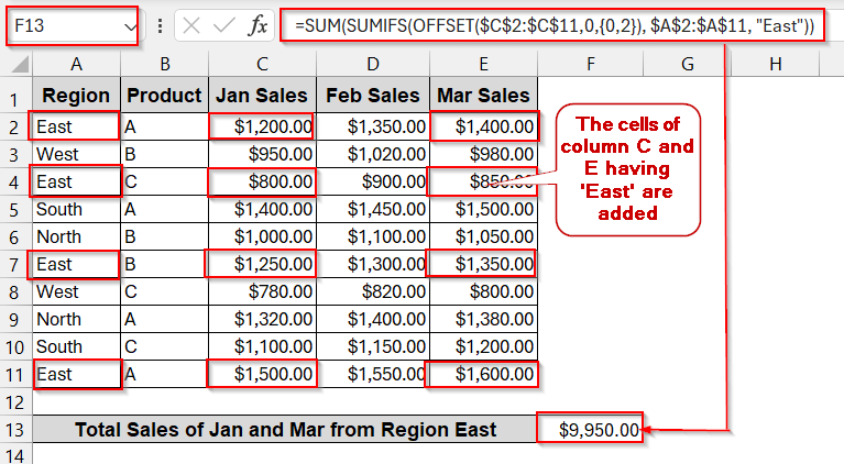
In this method, the total sales for only the months of January and March will be found in the ‘East’ region.
Steps:
➤ Open the worksheet and identify the columns to add and the conditions.
➤ Select the cell to write the formula.
➤ Enter the formula in the desired cell.
=SUM(SUMIFS(OFFSET($C$2:$C$11,0,{0,2}), $A$2:$A$11, "East"))
Here C2:C11 is the starting column, and the 0 represents the first one. The {0,2} represent the columns 0 (Jan Sales) and 2 (Mar Sales) that need to be added. The rest of the SUMIF formula is the same as before.
➤ Press Enter to get the result in the output cell.
Notes:
➨ OFFSET is a volatile function. This means this formula is recalculated every time the sheet changes and the values change.
➨ The array constant {} must match the column positions or the offset relative to the starting range. Otherwise, the formula won’t work.
Dynamic Column Selection and Sum with SUMIFS & INDEX Functions
INDEX works similarly to the OFFSET. It has the same capabilities to use the non-adjacent columns using array constants, though their syntax can vary a bit. Despite these, the sheer difference is that the INDEX formula is more robust, dynamic, and is best suited for large data.
Like the previous method, we will find the total sales for January and March from the ‘East’ region.
Steps:
➤ Open the dataset, choose the columns you want to add, and select the criteria.
➤ Select an empty cell to write the result of the total sales.
➤ Write the formula below of SUMIFS with INDEX.
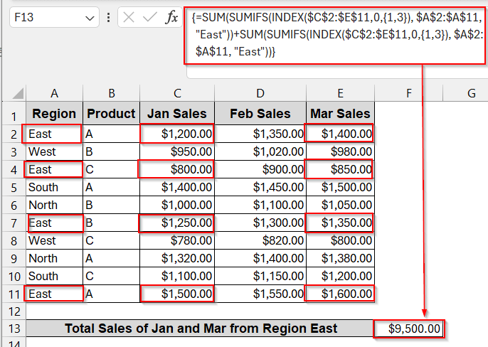
=SUM(SUMIFS(INDEX($C$2:$E$11,0,{1,3}),$A$2:$A$11,"East"))
Here, C2:E11 is the column range, {1,3} indicates the first and third columns, and the criteria filter the values with the rows having ‘East’.
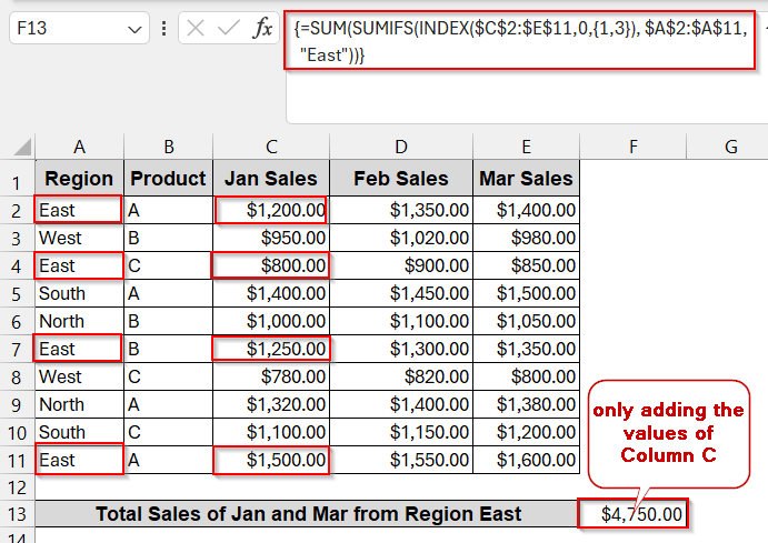
➤ As you can see, the formula finds the sum of the first column only, but does not add the rest. For this, we will add this formula again to itself –
=SUM(SUMIFS(INDEX($C$2:$E$11,0,{1,3}), $A$2:$A$11, "East")) + SUM(SUMIFS(INDEX($C$2:$E$11,0,{1,3}), $A$2:$A$11, "East"))
➤ Press Enter to get the output in the required cell.
Notes:
For many versions of Excel, this formula might not work simply by pressing Enter. If you see #Value instead of the result, try pressing Ctrl + Shift + Enter .
Creating a VBA Function for Multi-Column Summation
To reduce the manual hurdles of the SUMIFS formula and its frequent use, you can create a VBA function for this. By creating your own formula in a VBA script, you can automate the calculation. You do need this while dealing with large data that needs to be updated over time.
Steps:
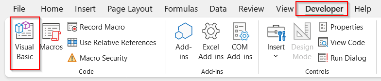
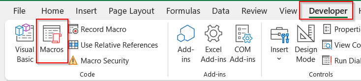
➤ Go to the Developer tab -> Visual Basic.
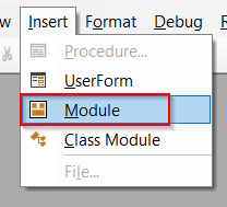
➤ It will launch the VBA Editor. Click on the Insert tab in the new window and choose Module.
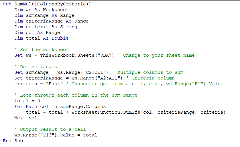
➤ Paste the following VBA code in the empty space-
Option Explicit
Sub SumMultiColumnsByCriteria()
    Dim ws As Worksheet
    Dim sumRange As Range
    Dim criteriaRange As Range
    Dim criteria As String
    Dim col As Range
    Dim total As Double
    ' Set the worksheet
    Set ws = ThisWorkbook.Sheets("Sheet1") ' Change to your sheet name.
    ' Define ranges
    Set sumRange = ws.Range("C2:E11") ' Multiple columns to sum
    Set criteriaRange = ws.Range("A2:A11") ' Criteria column
    criteria = "East" ' Change or get from a cell, e.g., ws.Range("H1").Value
    ' Loop through each column in the sum range
    total = 0
    For Each col In sumRange.Columns
        total = total + WorksheetFunction.SumIfs(col, criteriaRange, criteria)
    Next col
    ' Output result to a cell
    ws.Range("H2").Value = total
End Sub
➤ Press Ctrl + S to save the VBA Macros so they can be reused later.
➤ Close the window and go to the Developers tab. Click on Macros beside Visual Basic.
➤ Open the Macros window, and you will find the name of the formula you just created.
➤ Select the formula and click on Run.
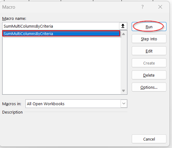
➤ This will automatically calculate the total sales from January to March based on the region ‘East’.
Notes:
➨Replace the sheet name on line 9 with your sheet name –
Set ws = ThisWorkbook.Sheets(“Sheet1”) ‘ Change to your sheet name
➨Replace the ranges with your ranges from lines 11 and 12.
Set sumRange = ws.Range(“C2:E11”) ‘ Multiple columns to sum
Set criteriaRange = ws.Range(“A2:A11”) ‘ Criteria column
➨Set the criteria as per your requirement in line 13.
criteria = “East”
➨You can also give the cell reference if you want. Then, the VBA script of line 13 will look like this:
ws.Range(“H1”).Value (where H1 holds the value that works as the criteria)
Alternative Methods to SUMIFS for Summing Multiple Ranges
Using SUMPRODUCT to Sum Multiple Columns by Criteria
SUMPRODUCT is the most-used alternative to SUMIF. It has a similar formula syntax to SUMIF. But the good thing is that, unlike the prior one, SUMPRODUCT can sum multiple column values singly. Without the help of any columns.
Steps:
➤ Open the sheet and identify the columns that you want to add.
➤ Select a cell to write the output.
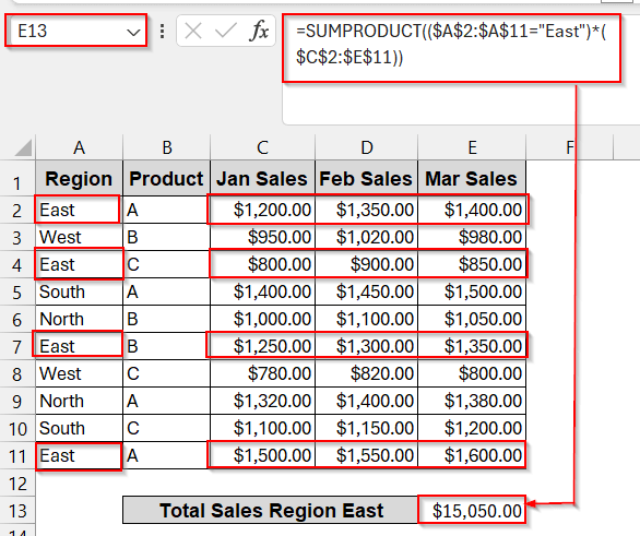
➤ In the selected cell, write the formula below –
=SUMPRODUCT(($A$2:$A$11="East")*($C$2:$E$11))
➤ Press Enter to display the result in the desired cell.
Using Power Query for Conditional Multi-Column Totals
Power Query is the no-formula way to achieve results similar to those of SUMIFS. All you have to do is group your cells by a specific condition and sum them up. It will be a lifesaver when working with recurring reports and huge datasets that need to be reloaded multiple times in a day.
With this method, we will find the total sales in the ‘East’ region.
Steps:
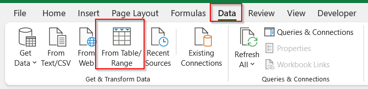
➤ Select any cell of the table and go to the Data tab. Click on From Table/Ranges.
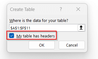
➤ A dialog box appears for the table range. Check the box. My table has headers, so click OK.
➤ This will load the data into the Power Query Editor window.
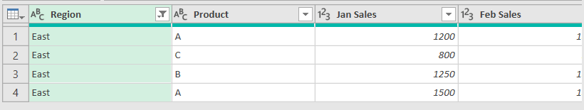
➤ In the Region arrow button, unselect all rows, and only select ‘East’.
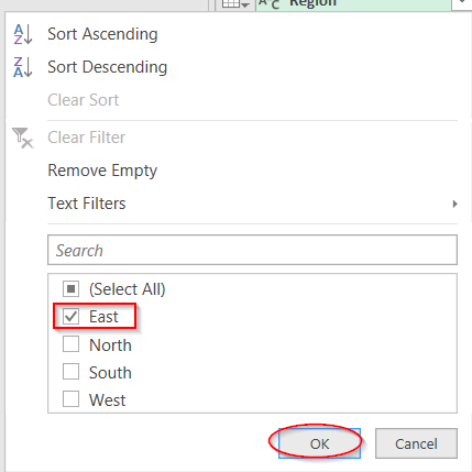
➤ This will only show the rows in the ‘East’ region.
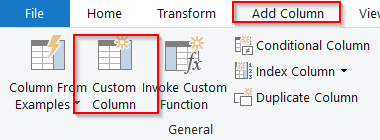
➤ Now, to add a new column, I’m going to the Add Column tab. Select Custom Column from the General group.
➤ In the Custom Column window, give a preferred name in the name field. In the formula box, enter the sum of the columns that you want to add.
[Jan Sales] + [Feb Sales] + [Mar Sales].
Here, Jan Sales, Feb Sales, and Mar Sales are the column names that need to be added.
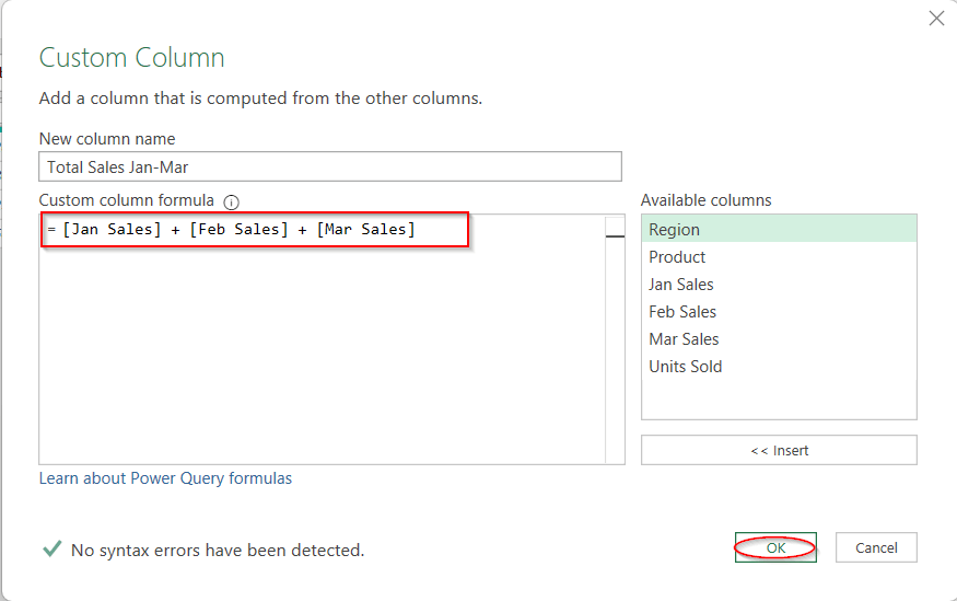
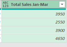
➤ By clicking OK, a new column will be created with the sum of the three columns for each row.
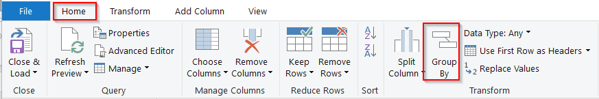
➤ To sum up all the columns in this new column, go to Home -> Group By.
➤ In the Group By window, select Advanced. Remove any rows below. Give the name of the new Groyp By column, select the Operation to Sum, and the Column to the new column (Total Sales Jan-Mar)
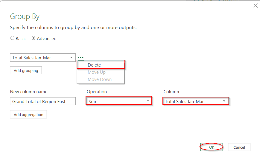
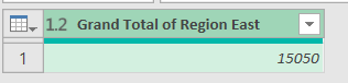
➤ Click OK to generate a new column with the total sum in the Power Query Editor window.
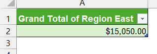
➤ Go to the Home tab and click on Close and Load to open a new worksheet with the total sum of the columns.
Notes:
Power Query does not update the data automatically. Click on Refresh to dynamically get updated data.
Frequently Asked Questions (FAQs)
Can SUMIFS handle multiple sum ranges directly?
SUMIFS does not support multiple column ranges. It only sums one column based on the criteria. To overcome this, we need to combine it with other formulas or write SUMIFS separately for each column and sum them up.
Can I sum non-contiguous columns with SUMIFS?
As SUMIFS cannot sum multiple columns, it can not sum non-contiguous ones. However, using OFFSET or INDEX with the SUMIFS, you can actually sum columns that are not adjacent.
What’s the difference between SUMIFS and SUMPRODUCT?
SUMIFS is dependent and works on a logical or conditional approach. On the other hand, SUMPRODUCT is based on mathematical calculations. That’s why SUMIF does not have the flexibility to sum a wide range of columns, unlike SUMPRODUCT.
Is there a way to SUMIF this dynamically without updating formulas?
You can dynamically update the formula and the values in SUMIFS by referencing the criteria. Instead of writing the criteria by hand, you can give the cell reference to make it more dynamic.
How to use SUMIFS with three criteria?
To use the SUMIFS formula with three criteria, you can write each criterion following the criteria range.
=SUMIFS(sum_range, criteria_range1, criteria1, criteria_range2, criteria2, criteria_range3, criteria3)
Concluding Words
Whether you want the simplicity of Excel or the automation of the advanced tools, you can work with SUMIFS in any workflow. With the formula-based approach of SUMIFS, SUMPRODUCT, BYCOL, and OFFSET, you can handle multiple and non-adjacent columns with wide ranges of criteria. On the other hand, the non-formula-based Power Query or the instant automation of VBA offers far better and easier solutions for the tech-savvy Excel lovers. With all these methods in hand, you’re not solving a problem – you are building a toolkit that works for any dataset size and Excel version.