Filtering a pivot table by a date range helps find the exact data you need for an analysis. Imagine you need to find the sales data for 10 days of a specific month. Filtering will help you extract the data using the date range. There are multiple ways to do this in Excel. Depending on what you would like to achieve, you can choose the approach you like best. In this article, we will go through all of the methods that can be used to filter the date range in a pivot table.
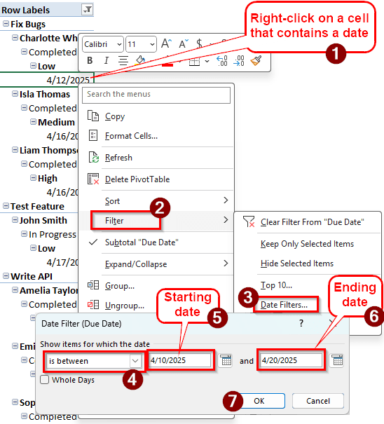
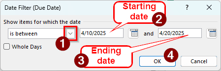
➤ In the pivot table, right-click on a cell that contains a date.
➤ Go to Filters > Date Filter.
➤ Choose “is between” from the dropdown on the left, and enter the starting and ending dates afterwards.
➤ Press OK to filter the pivot table.
That is the default method provided by Excel to filter a date range. However, it may not be sufficient for all cases. If you are interested in knowing more about filtering using a date range, keep reading the article to learn more methods to do this.
Using Date Filters to Filter the Pivot Table
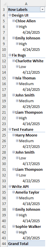
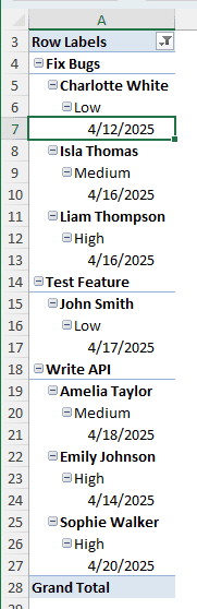
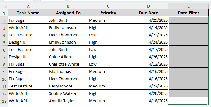
We have a small dataset that we will use for the tutorial to demonstrate the methods of filtering a pivot table with a date range. In the dataset, we have some task assortment data. There are task names, names of the people those tasks were assigned to, the priority of those tasks, and the due dates. We will filter the pivot table using a date range.
➤ In the pivot table, find a cell that has a date in it. We are selecting the A7 cell.
➤ Right-click on that cell, and go to Filter > Date Filters.
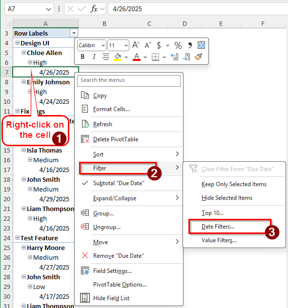
➤ A small window will open with filtering options. In the dropdown menu on the left, select “is between”. In the middle, write the starting date ( 4/10/2025 in this case ), and in the right, write the ending date ( 4/20/2025 here). Press OK to confirm.
➤ Now the pivot table only shows data from the dates between 4/10/2025 and 4/20/2025.
Filtering Date Range Using the Timeline
In the pivot table, we can add a timeline that simplifies the filtering process. We can insert a timeline and select the dates we want to see in the pivot table, and dynamically change it whenever we want. Follow the steps below to apply this method to your dataset.
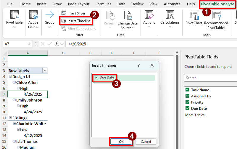
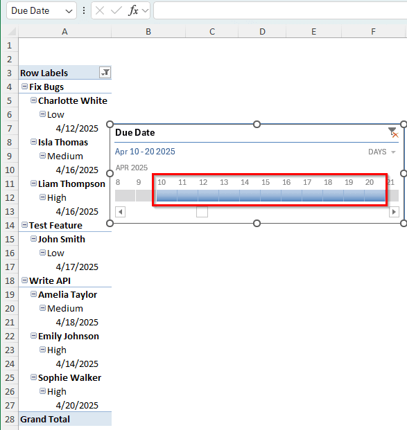
➤ When you have a cell of the pivot table selected, go to the PivotTable Analyze tab.
➤ From the Filter section, select Insert Timeline.
➤ In the Insert Timelines window, select Due Date (This is for this dataset. You will have to select the date category according to the name it has on your dataset). Click on OK to add the timeline.
➤ In the timeline, select April as that’s the month we want to filter the days in. Then, change the filter to DAYS.
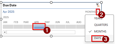
➤ Using your mouse, select 10 to 20 in the days portion. The pivot table should now be filtered with that date range.
Changing the Source Dataset to Filter the Date Range in the Pivot Table
We can make changes to our source dataset and create a new pivot table to filter it using our chosen date range. This method requires a lot of work, so it’s only recommended when you cannot use the other methods for some reason, or you want the filter to be added to your dataset as well. Follow the steps below:
➤ Go to the source dataset, and add a new column called Date Filter.
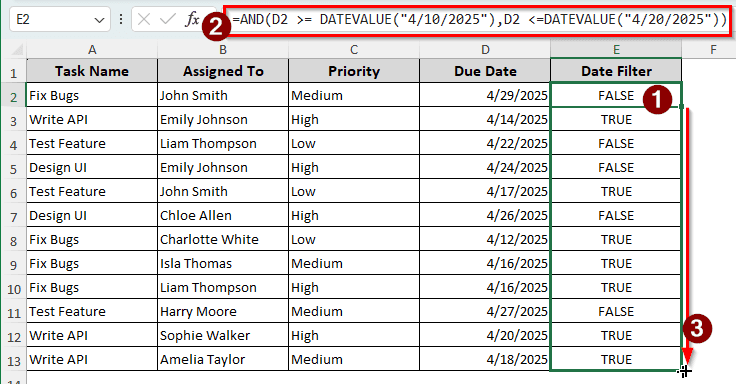
➤ In the E2 cell of the dataset, write the following formula, then autofill until E13.
=AND(D2 >= DATEVALUE("4/10/2025"),D2 <=DATEVALUE("4/20/2025"))
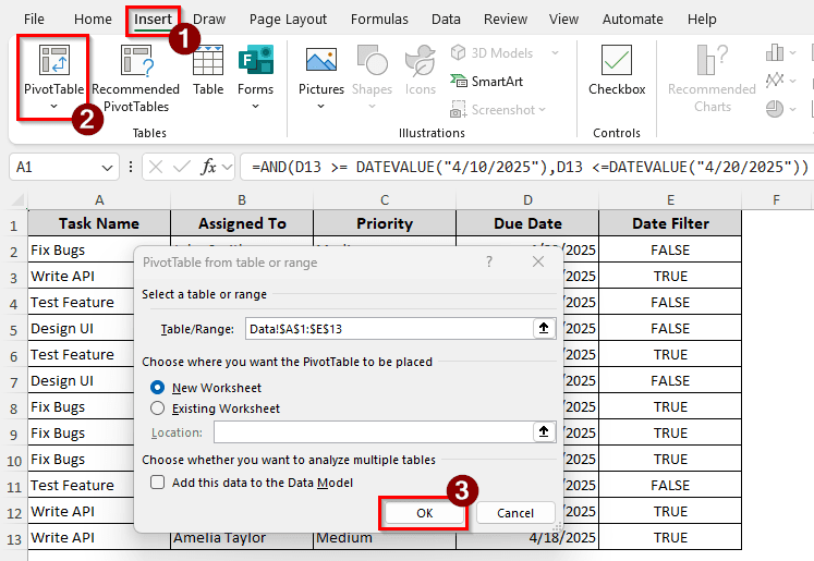
➤ Create a new pivot table using the A1:E13 data range. Select the data, and go to the Insert tab of the ribbon. Then, select PivotTable. In the new window, press OK to create the pivot table.
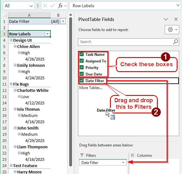
➤ In the new pivot table, select all the fields to add them to the table, but drag the Date Filter field to the Filters area.
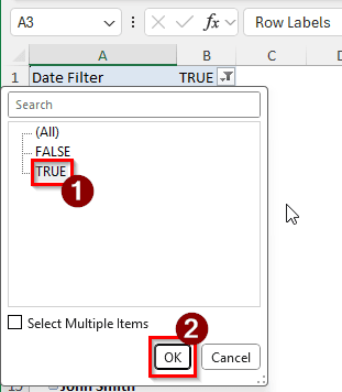
➤ Now that the Date Filter is added to the pivot table, choose True from the dropdown of the filter and click on OK.
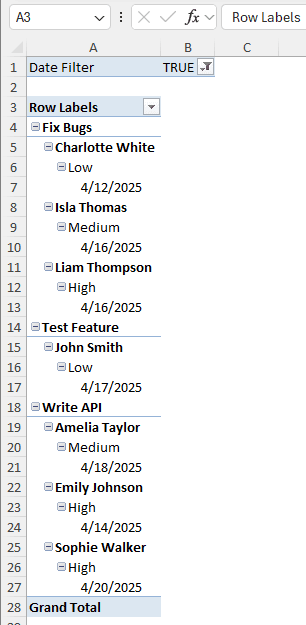
➤ Here is how the pivot table should look afterwards:
Manually Selecting the Dates of the Range
If everything else fails, this is the method that takes the most time and is pretty inefficient in general. But it works, so it’s effective.
➤ Move the Due Date field to the Filters area.
➤ Open the dropdown menu from the B1 cell.
➤ Check the box that says Select Multiple Items.
➤ Check all of the boxes that contain the dates from your chosen range. Click OK to confirm.
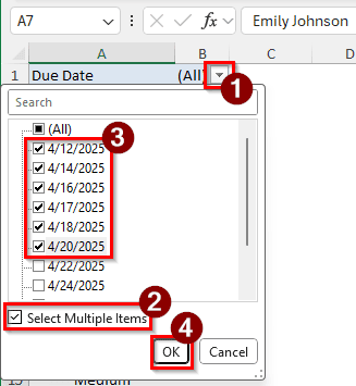
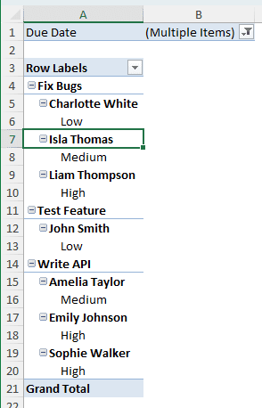
➤ The pivot table should be filtered now, although the dates won’t show up.
Frequently Asked Questions
How to get the date in dd mm yyyy format in pivot?
It’s the same as doing it in a normal table. Select the target cell, and go to the Number section of the Home tab. From there, open the dropdown menu, select More Number Formats. A new window will open, and you can select the desired format from there.
How to get dates in pivot table values?
In the PivotTable Fields section, the dates are usually kept in the Rows area. Click on the field that has the dates, and select Move to Values. The dates will show up in Values as count now.
Why is my pivot table not grouping dates?
Check the source dataset to see whether the dates are formatted correctly or not. If any cell that was supposed to include a date does not include one, the pivot table will not group the category. You must also make sure that the dates are called Date in the Number section of the Home tab. If it’s called Text, change it. Once you have completed all of these, create a new pivot table with the existing data range.
Why is the date filter not working in a PivotTable?
The pivot table is not seeing the dates as dates for some reason. The possible explanation for this is that the dates in the source dataset are not formatted as dates. Go to your source data range, change the number format of the cells that contain dates, and recreate the pivot table.
What is the formula for dates in Excel?
The DATE formula can be written as follows:
=DATE(A1,B1,C1)
Here, A1 refers to a cell that contains the year, B1 refers to the month, and C1 refers to the day.
Wrapping Up
In this article, we have learned how to filter a pivot table using a date range. If you have read the tutorial and followed along with us, you know all four methods that you can use to filter the pivot table. Download the practice file we used to write this tutorial to check the dataset for yourself. Stay tuned until next time.