Pivot Tables in Excel are used for summarizing and analyzing large datasets. A common challenge arises when you want to group several column fields under a single category. When you try to do this directly, it often results in a “Cannot group that selection” or the Group selection is greyed out.
In this article, we will guide you through several methods to group columns in Pivot Table without encountering errors. We will start with a sample dataset and Pivot Table setup, then proceed with the grouping techniques.
To group columns in Pivot Table, here is one simple solution by using the PivotChart Wizard feature.
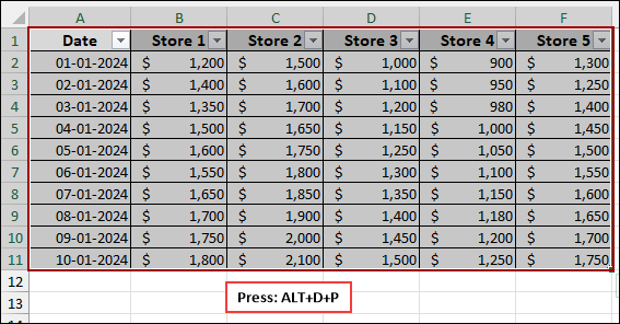
➤ Select the table and press Alt + D + P to open PivotChart Wizard.
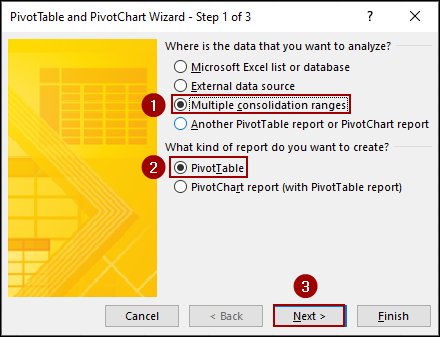
➤ Click Multiple consolidation ranges > PivotTable > Next.
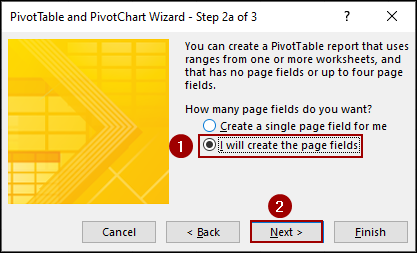
➤ Select I will create the page fields > Next.
➤ Add the range and click Next.
➤ Choose New Worksheet > Finish.
➤ Select the column headings you want to group (e.g., Store 1, Store 2, and Store 3).
➤ Go to the PivotTable Analyze tab and choose Group Selection to group columns in Pivot Table.

Using Calculated Field to Group Columns in Pivot Table
The Calculated Field feature is ideal for simple grouping scenarios where you want to combine the values of multiple column fields. This approach does not physically group the columns but introduces a new column that holds the grouped totals.
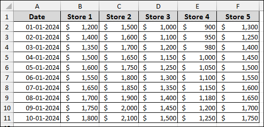
To demonstrate these methods, we will use a sample dataset showing daily sales for five different stores.
First, we will convert the data into an Excel Table, which is the best practice for working with Pivot Tables and Power Query.
To convert the data into a Table.
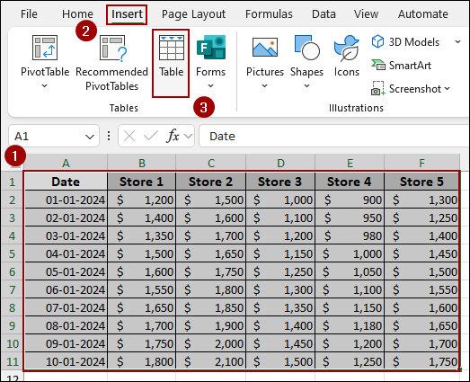
➤ Select the dataset (A1:F11).
➤ Go to the Insert tab on the ribbon.
➤ Click the Table option.
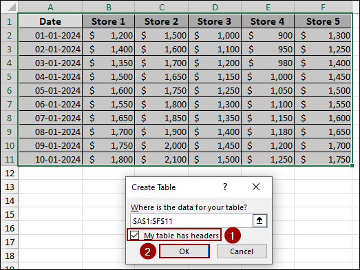
In the Create Table dialog box,
➤ Ensure the data range is correct.
➤ Checkmark My table has headers.
➤ Click OK.
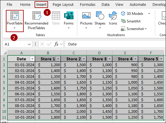
Now that the data is a proper table, we can create the Pivot Table.
➤ Go to the Insert tab.
➤ Click the PivotTable button.
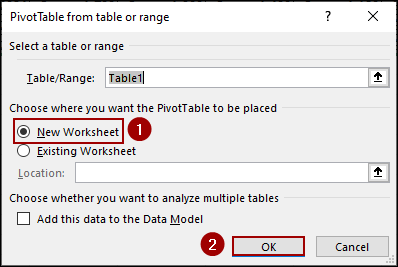
➤ In the new dialog box, select New Worksheet to place the Pivot Table on a new sheet.
➤ Click OK.
The initial Pivot Table is now created. Suppose we want to group Store 1, Store 2, and Store 3 into North Sales, and Store 4 and Store 5 into South Sales. To begin, make sure your Pivot Table fields are set up (e.g., Date in Rows, Store 1-5 in Values).
➤ Click inside your Pivot Table.
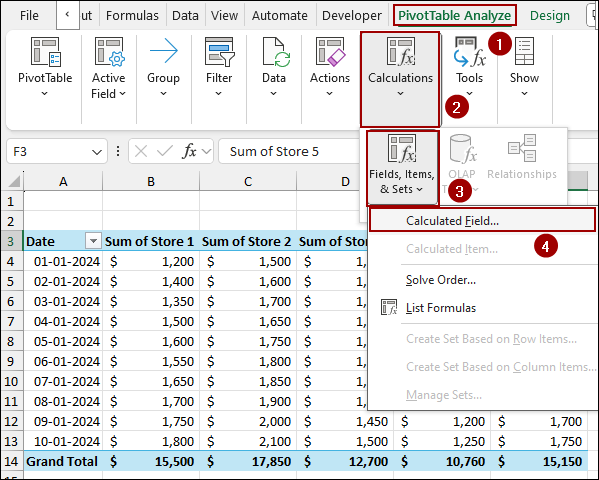
➤ Navigate to the PivotTable Analyze tab on the ribbon.
➤ In the Calculations group, click on Fields, Items, & Sets.
➤ From the dropdown menu, select Calculated Field.
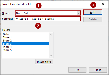
In the Insert Calculated Field dialog box:
➤ In the Name box, type North Sales.
➤ In the Formula box, enter the formula to sum the desired stores.
='Store 1' + 'Store 2' + 'Store 3'
You can double-click the field names in the Fields list to insert them.
➤ Click Add.
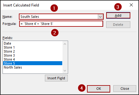
Thus, the North Sales field will be added to the Pivot Table field. Now, let’s add the South Sales field.
➤ Change the Name to South Sales.
➤ In the Formula box, enter the formula.
='Store 4' + 'Store 5'
➤ Click Add.
➤ Click OK to close the dialog box.
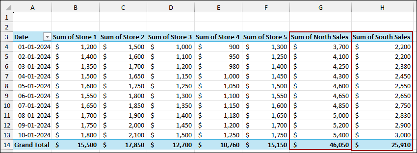
The Pivot Table now includes the two new calculated fields: Sum of North Sales and Sum of South Sales. These columns appear alongside the original store columns, effectively grouping the data by region based on the calculation.
Utilizing PivotChart Wizard Feature to Group Columns
This method uses a hidden feature of Excel to create a Pivot Table that is group-friendly. By using the Multiple consolidation ranges option in the PivotChart Wizard, Excel creates a different kind of Pivot Cache, which allows direct column grouping.
➤ Select the data range (A1:F11) on your original data sheet.
➤ Press the shortcut keys Alt + D + P to open the PivotTable and PivotChart Wizard.
In the first step:
➤ Select Multiple consolidation ranges.
➤ Choose PivotTable for the report type.
➤ Click Next.
In the next step:
➤ Select I will create the page fields.
This setting is the main key to the functionality.
➤ Click Next.
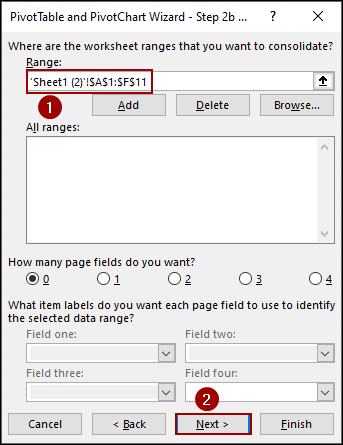
➤ Select the range (‘Sheet1 (2)’!A1:F11).
➤ Click Next.
➤ Choose New worksheet to place the new Pivot Table.
➤ Click Finish.

Your new Pivot Table will appear with the store columns in the Column Labels area.
➤ Select the column headings you want to group (e.g., Store 1, Store 2, and Store 3).
➤ Go to the PivotTable Analyze tab.
➤ In the Group area, click Group Selection.
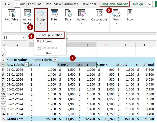
The selected columns will be grouped under a new field called Group1. Here, we named it North Sales.
Now, we will group the remaining columns.
➤ Select the next set of column headings (e.g., Store 4 and Store 5).
➤ Go to the PivotTable Analyze tab.
➤ In the Group section, click Group Selection.

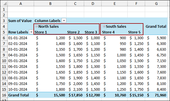
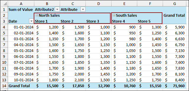
After that, rename the group as South Sales. The resulting Pivot Table now clearly shows the store sales grouped under the new regional headers, demonstrating successful column grouping.
Using Power Query Tool for Grouping Columns
The most flexible method is to use Power Query’s Unpivot feature, which is compatible with complex or dynamically changing data. This transforms the column headers into row data, allowing you to create groups in a new column before building the Pivot Table.
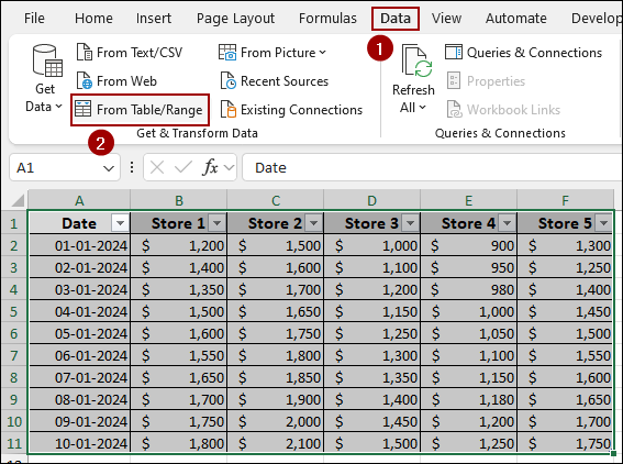
➤ Click anywhere inside your data table.
➤ Go to the Data tab.
➤ In the Get & Transform Data group, click From Table/Range.
This opens the Power Query Editor. In the Power Query Editor:
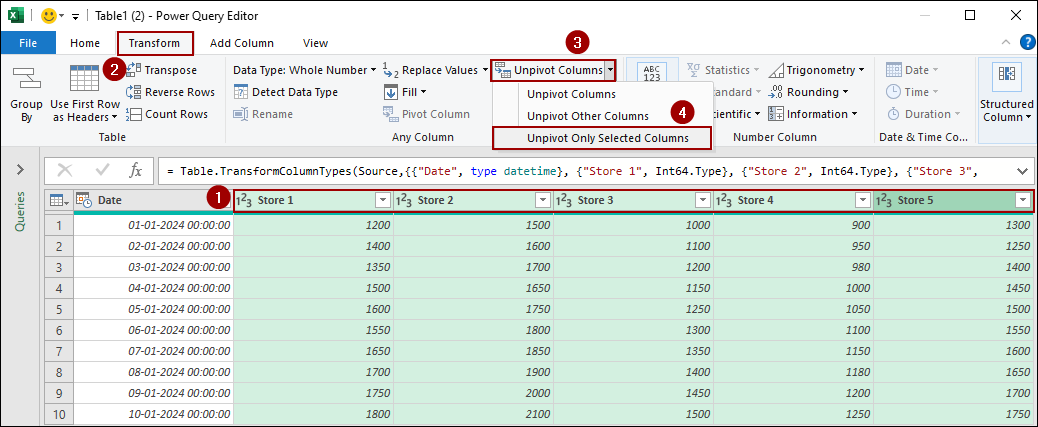
➤ Select the columns you want to unpivot (the store columns, Store 1 through Store 5).
➤ Go to the Transform tab.
➤ Click the dropdown under Unpivot Columns.
➤ Select Unpivot Only Selected Columns.
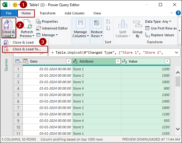
This action transforms the store columns into two new columns: Attribute (containing the store names) and Value (containing the sales figures).
➤ Go to the Home tab.
➤ Click the dropdown next to Close & Load.
➤ Select Close & Load To.
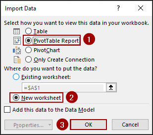
In the Import Data dialog box:
➤ Choose the option PivotTable Report.
➤ Select New worksheet.
➤ Click OK.
The Pivot Table will be created based on the transformed data.
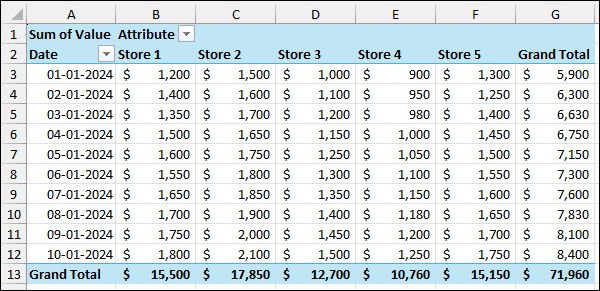
Similar to the previous method, group the data of Stores 1, 2, and 3 as North Sales, and Stores 4 and 5 as South Sales. Finally, we have successfully grouped columns in a Pivot Table with the stores grouped under the new headers.
Frequently Asked Questions
Can I group dates that appear as column headers in a PivotTable?
Yes. Right-click on any date in the column labels, click Group, and choose Days, Months, Quarters, or Years. Excel will automatically summarize your data into those periods.
Why is the Group option greyed out in my PivotTable?
This usually happens if your column labels contain blank cells, text values when Excel expects numbers/dates, or if your PivotTable is based on Power Pivot data models, where manual grouping is not allowed.
Can I group PivotTable columns dynamically without adding a helper column?
No, PivotTables don’t allow “custom formulas” for column grouping. The only dynamic ways are through date grouping, number grouping, or using Power Query to reshape data before building the PivotTable.
Concluding Words
Above, we have explored three different methods to group columns in Pivot Table. For quick, calculative grouping, Calculated Fields are the best fit. For a traditional Pivot Table layout that allows for direct grouping, the PivotChart Wizard is an excellent feature. Finally, for the most flexible solution, the Power Query Unpivot technique is highly recommended. By using these methods, you can overcome the common grouping errors in Excel. If you have any questions, please don’t hesitate to let us know in the comments section below.