
When we work with large datasets in Excel, it can get messier if we try to analyze the row data directly. That’s where we can use a summary report because it organizes the scattered information into a clear format. And so, it helps us to track performance, compare categories, and highlight key trends of our dataset easily and quickly.
Suppose you are analyzing sales data for multiple regions and products. Now, if you go through hundreds of rows to find the sales or the best and low-performing products of each region, it will take a lot of time and effort. Instead, you can make a summary report that will show you the total sales by region or the average sales per product instantly.
In this article, we will learn different methods to create a summary report in Excel, including using the PivotTable and the SUMIF function.
➤ First, select the whole dataset, i.e., cells A1:C9.
➤ Then, go to the Insert tab on the upper ribbon and click PivotTable in the Tables group.
➤ Now, a pop-up window will appear. Choose whether you want the PivotTable in a New Worksheet or an Existing Worksheet, then click OK.
➤ Then, in the PivotTable Fields panel, drag City to the Rows area and Product to the Columns area.
➤ Drag Sales to the Values area. By default, Excel will calculate the Sum of Sales
➤ Now, you’ll see a summary report where each city is listed in rows, products are listed in columns, and the sales values are summarized.

Create a Summary Report in Excel Using the PivotTable
A PivotTable is one of the most powerful tools in Excel for creating summary reports. It allows you to quickly reorganize, group, and calculate large datasets without using complex formulas, giving you flexibility to analyze your data from different angles..
We will use the dataset below to explain how you can create a summary report in Excel with the PivotTable.
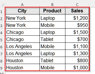
This is a sales dataset of a few products across some different cities.
Steps:
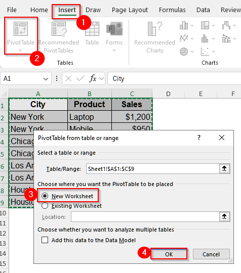
➤ First, select the whole dataset, i.e., cells A1:C9.
➤ Then, go to the Insert tab on the upper ribbon and click PivotTable in the Tables group.
➤ Now, a pop-up window will appear. Choose whether you want the PivotTable in a New Worksheet or an Existing Worksheet, then click OK.
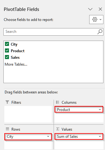
➤ Then, in the PivotTable Fields panel, drag City to the Rows area and Product to the Columns area.
➤ Drag Sales to the Values area. By default, Excel will calculate the Sum of Sales.
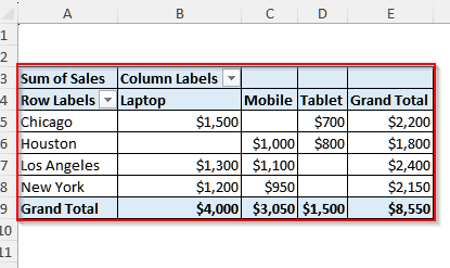
➤ Now, you’ll see a summary report where each city is listed in rows, products are listed in columns, and the sales values are summarized.
Create a Summary Report in Excel Using the SUMIF Function and Advanced Filter
The SUMIF function is very useful when we want to create a quick summary report without setting up a PivotTable. It allows us to add numbers in a range that meet specific criteria, such as sales by city or totals for a particular product.
To explain how you can create a summary report in Excel using the SUMIF function, we will use the dataset below.
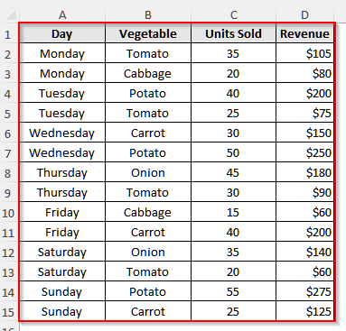
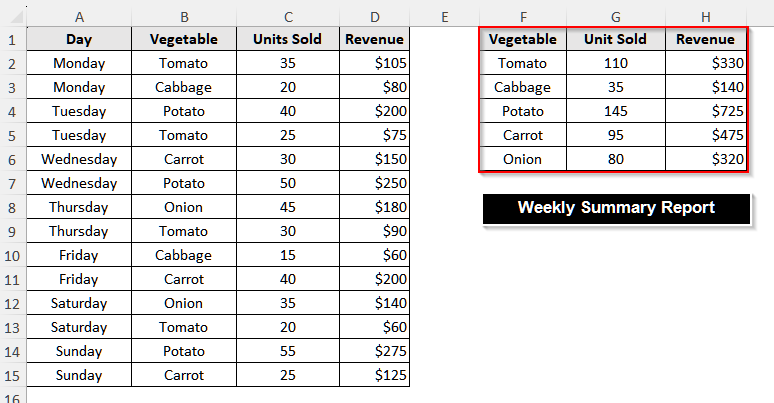
This dataset is a weekly report from a small grocery store. It contains the dates, vegetable names, units sold, and corresponding revenues. We will create a summary report to show the total units sold and the revenue generated by each vegetable during the week.
Steps:
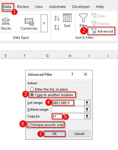
➤ First, select the Vegetable column, i.e., B1:B15.
➤ Then, go to the Data tab, and click on Advanced under the Sort & Filter group.
➤ Now, choose Copy to another location under the Action field.
➤ Then, to set the List range, select the range of vegetable names. Or, you can manually write $B$1:$B$15 in the List range box.
➤ Now, in the Copy to box, select any empty cell. For our dataset, we will write F1.
➤ Tick the Unique records only option and click OK.
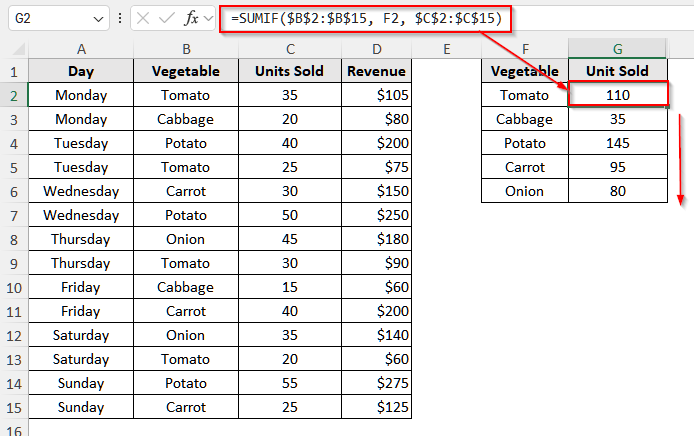
 ➤ Now, we have the unique vegetable names listed in column F.
➤ Then, click on cell G1 and write Unit Sold.
➤ Click on cell G2 and insert the following formula:
=SUMIF($B$2:$B$15, F2, $C$2:$C$15)
➤ Drag your cursor down to fill the cells for other vegetables to get the unit sold for each vegetable.
➤ Now, to calculate the total revenue for each vegetable, select cell H1 and write Revenue.
➤ Then, click on cell H2 and insert the following formula:
=SUMIF($B$2:$B$15, F2, $D$2:$D$15)
➤ Drag the cursor down to get the revenue for each vegetable.
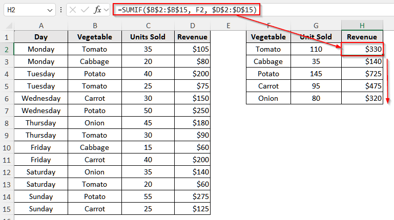
➤ Finally, the weekly summary report on vegetables is ready.
Frequently Asked Questions
Can I Schedule Data Refresh for Summary Reports in Excel?
Absolutely, you can. When your report is connected to an external data source such as a database, Power Query, or Power Pivot model, it usually updates over time. So, to schedule a refresh for your summary report in case of such a dataset, go to the Data tab, click on Connections, and then select Properties. In the Connection Properties window, choose the Refresh option and set the time as you want. You can also set it to refresh the data when opening the file.
How Do I Use a Template for Summary Reports in Excel?
To use a template for summary reports in Excel, first go to File and select New. Then, in the box Search for online templates, write Summary report or any keyword you are looking for. Finally, select a template that seems suitable and click Create. Then replace the sample data with your own while keeping formulas and formatting intact..
How Can I Prepare My Data For a Summary Report in Excel?
To prepare your data for a summary table, first clean the data by removing duplicates, fixing typos, filling in or deleting missing values, and keeping the formatting consistent across each column. This will ensure your summary report will be error-free and accurate.
Wrapping Up
In this article, we learned two different ways to create a summary report in Excel, including using the PivotTable and a combination of the Advanced function and the SUMIF formula. Try out these two simple and easy methods. Reach out in case you have any inquiries or feedback.