What is Value Axis in Excel Chart & How to Customize It

The value axis in Excel is the one that represents numeric values in a chart.

In 2-D charts or graphs, this is usually the vertical or Y-axis. In some cases, it can be horizontal (X-axis) too. We use the value axis to plot and scale data points for measurement and comparison.

We will refer to the value axis as the Y-axis in this article, as this is the standard convention.

We will cover the charts that can’t have value axes, how to customize the scale in the value axes, how to change the values of the value axes, how to add or remove the gridlines in the value axis and how to add secondary value axis in a chart.

What is Value Axis in Excel Chart?

Value Axis is the axis on a chart that represents values or numbers.

The value axis represents the scale of values for the data points (for example, sales numbers, temperatures, percentages, etc.). In most Excel charts, it is the vertical or Y-axis. For Bar charts, it is the horizontal or X-axis.

Different charts can have different maximum and minimum values depending on the range of data. You can always modify them in Excel. You can also change the axis scale (logarithmic or linear) and display units (thousands, millions, etc.). Some charts can also contain ranges instead of values.

If the graph requires a vertical axis, Excel will create it automatically based on the data.

In addition, Excel will automatically determine the scale and the start-end point. You can always customize the scale to match your preferences.

In this section, we will touch on some of the customization processes of the value axis.

Steps to Access the Format Axis Pane:

➤ Access the Format Axis pane in one of the following ways.
➤ Double-click on the value axis.
➤ Select the axis and go to Format >> Format Selection.

➤ You will find different scale options under the Axis options. This is the column icon in the pane.

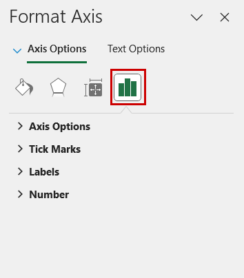
It has four sections inside it:

• Axis Options
• Tick Marks
• Labels
• Numbers

Changing Start and End Point of Axis:

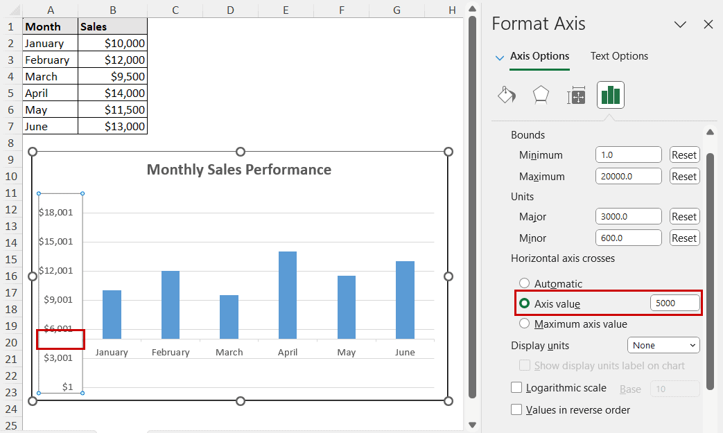
➤ Changing the Minimum and Maximum values under the Bounds of Axis Options will change the upper and lower limits of the graph.

Changing Axis Value Intervals:

➤ Changing the unit values will change the intervals on the axis.

Other Axis Value Options:

➤ The Horizontal axis crosses option checks where the X-axis will start on the vertical axis.

➤ The Logarithmic scale puts the axis on an exponential scale instead of linear.
This is helpful for a wide range of data.

➤ The Values in reverse order option flips the graph.

Tick Marks:

➤ The Major and Minor tick mark types can be set from the Tick Marks options.

Other Axis Formatting Options:

➤ You can change the Labels position under the Labels section.

➤ The Number section allows you to format the display of the values on the axis.

This section is dedicated to changing the values in the Value axis completely.

The value axis shows the values of the series. If we change the values of the series or the source of the series, the value axis will change accordingly.

Let’s say, we have the sales values in a graph from the data.

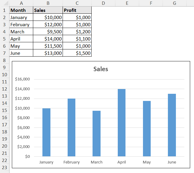
We want to display the profit values in the graph and the value axis now.

Steps:

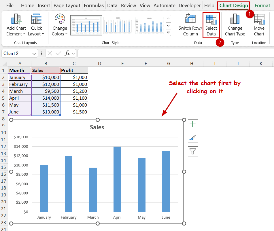
➤ Select the chart.
➤ Go to Chart Design >> Data (group) >> Select Data.

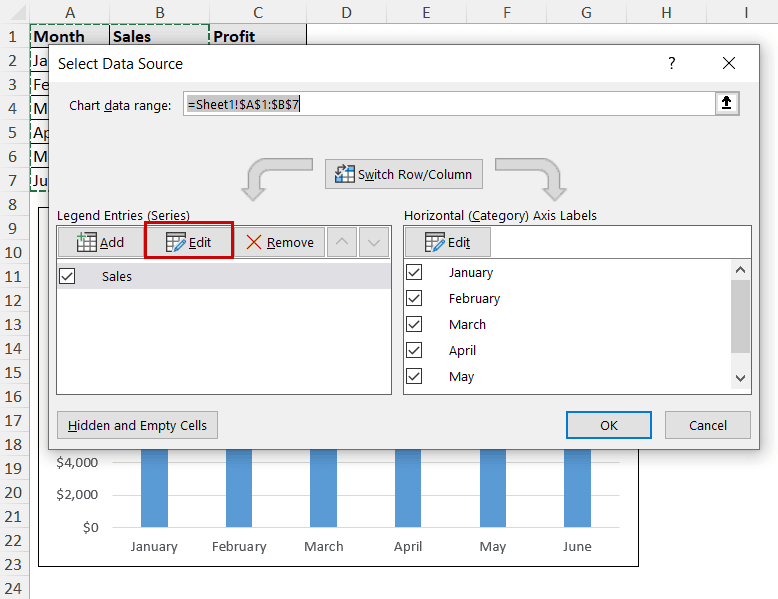
➤ Now select Edit under the Legend Entries section in the Select Data Source dialog box.

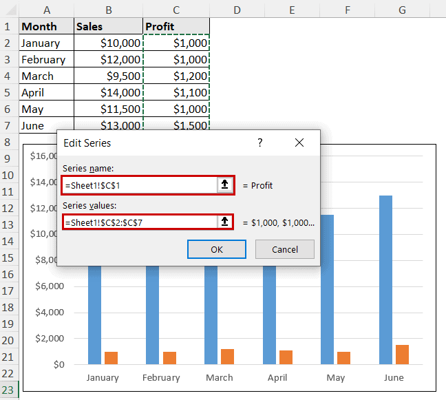
➤ Select the new series name and values in the Edit Series dialog box.

➤ Click OK and close all the boxes.

The Y-axis values will get updated to new values now.

Adding or Removing Gridlines

Gridlines are horizontal and vertical lines on the graph that intersect with each other to form a grid.

Gridline makes information easier to understand and improves precision when identifying trends. Value axis usually intersects with the horizontal lines to clearly represent the Y-axis values.

The gridline options are available in the Chart Elements button in Excel.

Steps:

➤ Select the chart.
➤ Click on the Chart Elements button that pops up on the upper-right of the chart.
This is the plus icon (+) on top of the buttons.
➤ Now select the Gridlines option from the list. Or, select the right arrow and choose the specific option you want to customize more.

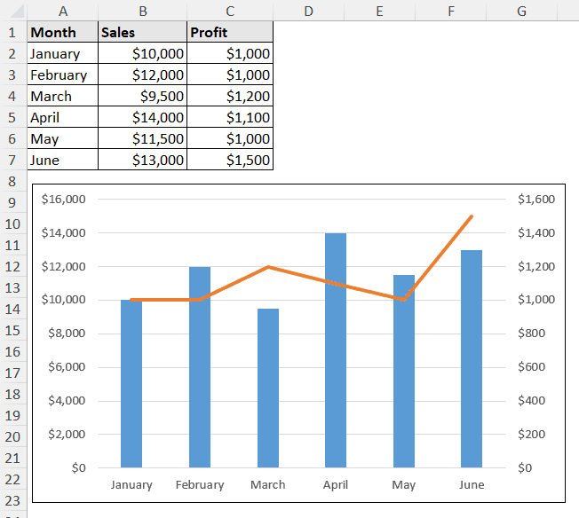
Adding Secondary Value Axis

The secondary Y-axis is available only in certain combo charts in Excel. You also need multiple series entries for the source too.

So, adding a secondary value axis is twofold: adding new series to the chart and adding secondary axis for it.

Steps to Add New Series:

➤ Select the chart.
➤ Go to Chart Design >> Data (group) >> Select Data.

➤ Click on Add under the Legend Entries in the Select Data Source dialog box.

➤ Now select proper series name and range source in the Edit Series dialog box.

➤ Click on OK after that.

Changing the Chart Type for Secondary Y-Axis:

➤ Select the chart.
➤ Go to Chart Design >> Type (group) >> Change Chart Type.

➤ In the Change Chart Type box,
➤ Select All Charts
➤ Select Combo from the chart types.
➤ Select a chart type from the right side of the dialog box.
➤ Check the secondary Y-axis series from the lower right of the box.

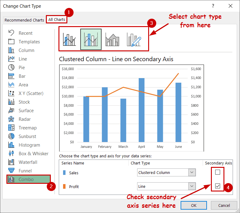
➤ Click on OK.

The chart will contain secondary value axis now.

Charts That Don’t Use Any Value Axis

Almost all of the charts contain the value axis.

Every chart consists of numeric points that make up the chart. But not every chart needs to show those values on an axis.

Usually, this happens when the chart structure is aligned to display the values in other ways.

Some of these charts include:

• Pie chart
• Doughnut chart
• Radar chart
• Treemap chart
• Sunburst chart
• Waterfall chart
• Funnel chart

Apart from these charts, all other charts can use the value axis. In fact, other charts might be confusing without the value axis.

FAQ

How do I make the value axis start at zero in Excel?

You can set the minimum value in the bounds to zero to start the value axis at zero.

Double-click on the axis values to open the Format Axis pane. You can find the bound’s minimum value option there.

How do I switch the Value Axis from the Y-axis to the X-axis in Excel?

To swap the X and Y axes, select the chart and select Chart Design >> Data (group) >> Select Data. Click on Edit under the Legend Entries section. Then manually insert the new X and Y values in the Edit Series dialog box.

Your data source must contain multiple numeric series to access the options in the Edit Series dialog box.

How do I add a title to the value axis in Excel?

To add a title to any axis, select the chart first. Then click on the Chart Elements button (the plus icon on the top-right). Check the Axis Titles option after that.

Conclusion

This article covers the discussion on the value axis in Excel. It includes different charts that do and don’t contain the value axis. How to change the scales in the value axis and how to change the values entirely.

The article also contains advanced customizations such as adding or removing gridlines and how to add a secondary value axis.

Feel free to download the practice file and let us know about your feedback.