Error bars in a data point are the measurement of the accuracy of the data. Different values for individual error bars indicate different margins of error for different data points.
An error bar indicates how much the correctness of the data fluctuates in the sample. It adds a degree of confidence to the data. Error bars are often based on statistical measures like standard deviation or standard error.
To add individual error bars in Excel,
➤ Calculate standard deviation or other measurements to add to the error bar.
➤ Open the Format Error Bars pane after selecting Chart Elements >> Error Bars >> More Options.
➤ Select Custom and click on Specify Value under Error Bar Options.
➤ Select the calculated values in the positive and negative fields of the Custom Error Bars dialog box.
In this tutorial, we will go over how to add individual error bars in Excel when you have multiple series. We will cover how to open the Format Error Bars pane in two ways. Then, how to use the customizable option from the pane to add error bar values to each series.
Download Practice WorkbookStep 1: Calculating Standard Deviation
We have the following dataset for the demonstration. It tracks the growth rate of plants across different weeks.
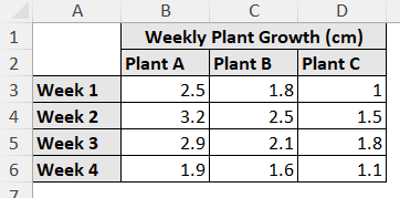
We need to calculate the standard deviation for each plant before adding the values as error bars.
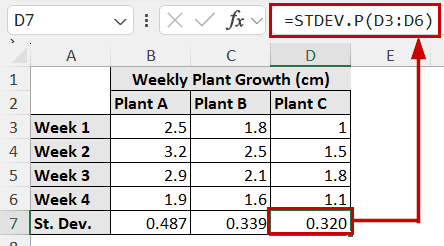
Excel offers the STDEV.P function to calculate the standard deviation from a range.
➤ Select a cell and use the formula: STDEV.P(range).
Step 2: Create a Chart
Next, select an appropriate chart where you want to insert the error bars.
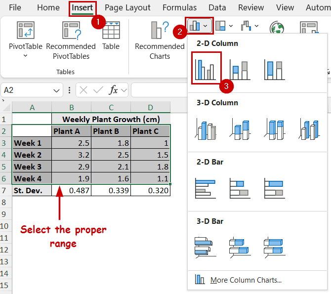
You need to select the appropriate range first (A2:D6). Otherwise, Excel will include the standard deviation values (B7:D7) in the chart too.
We are going to create a clustered column chart for the demonstration.
➤ Select the appropriate range (A2:D6).
➤ Go to Insert >> Charts (group) >> Insert Column or Bar Chart >> Clustered Column.
Step 3: Opening Format Error Bars Pane
Every customization option available for error bars is in the Format Error Bars pane.
We can open the Format Error Bars pane in two ways: using the Chart Elements button or the Chart Design tab.
Using the Chart Elements Button
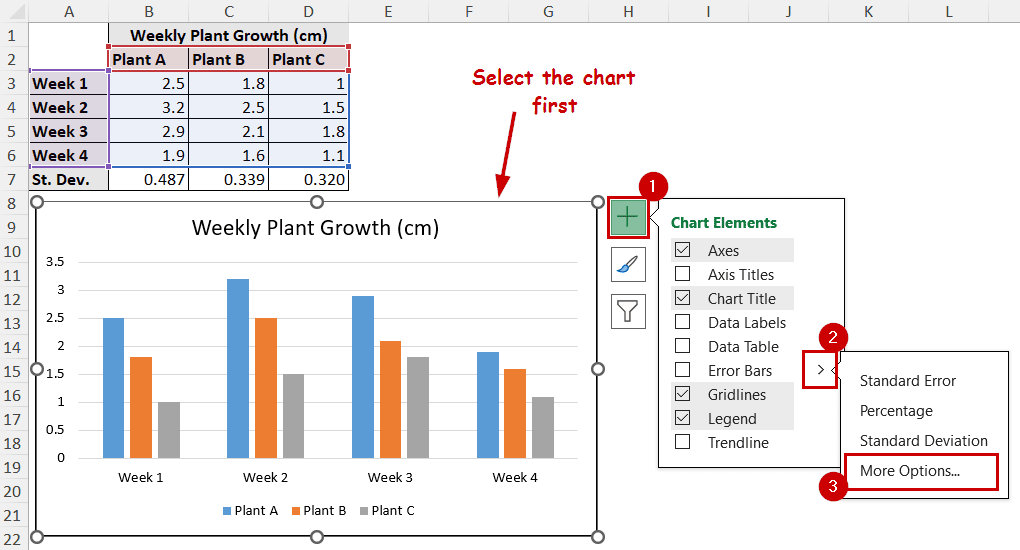
The Chart Elements button appears at the top-right of a chart after selecting the chart. It is the plus (+) icon on top of the buttons.
To open the Format Error Bars pane using the Chart Elements button,
➤ Select the chart.
➤ Go to Chart Elements >> Error Bars >> More Options.
➤ If you have multiple series, select a series.
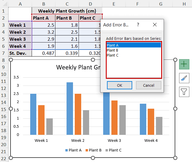
The Format Error Bars pane will open on the sheet.
Using the Chart Design Tab
Two new tabs are accessible in the ribbon after selecting a chart: Chart Design and Format.
The same options to add or modify chart elements are also available in the Chart Design tab. You can add error bars and modify them using this tab.
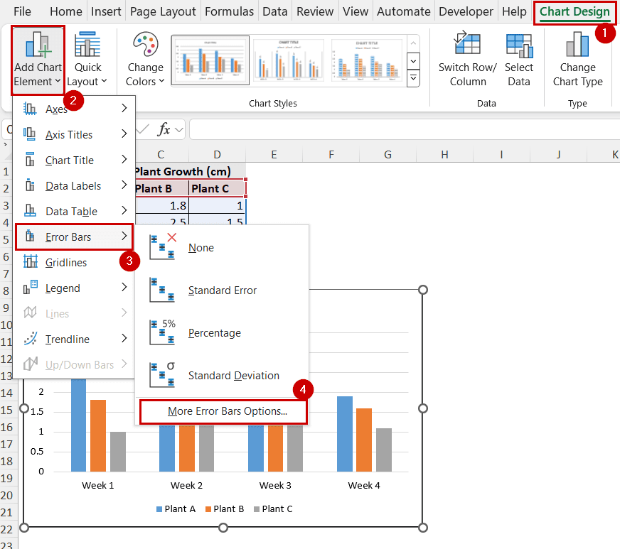
To open the Format Error Bars pane using the Chart Elements button,
➤ Select the chart.
➤ Go to Chart Design >> Chart Layouts (group) >> Add Chart Element.
➤ In the dropdown, select Error Bars >> More Error Bars Options.
➤ Select a series if you have multiple series.
Step 4: Select Individual Error Bar Values
Now it’s time to add the standard deviation value as a custom error value for the series.
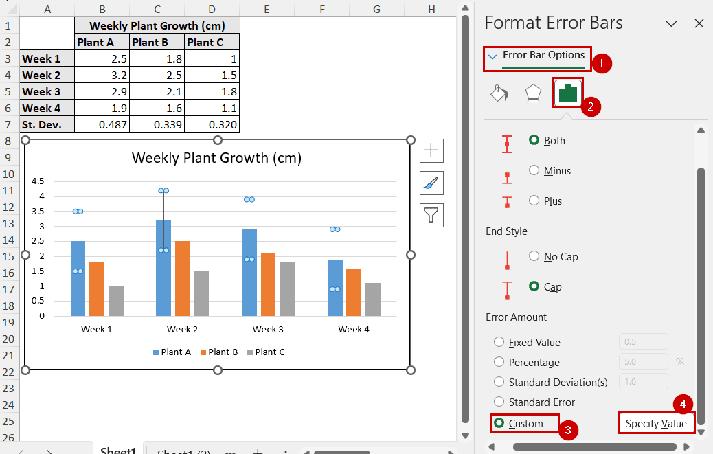
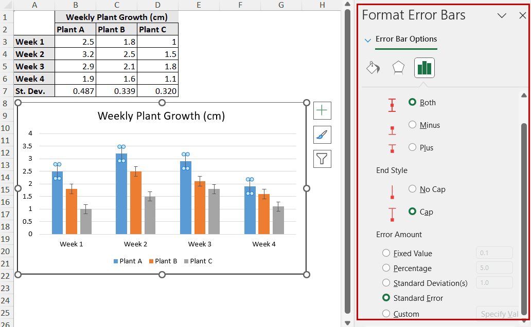
➤ Select Error Bar Options in the Format Error Bars pane.
➤ Select Custom in the Error Amount and click on Specify Value.
➤ Select standard deviation values in the positive and negative fields in the Custom Error Bars dialog box.
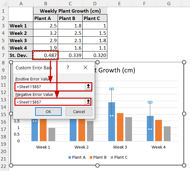
➤ Click on OK.
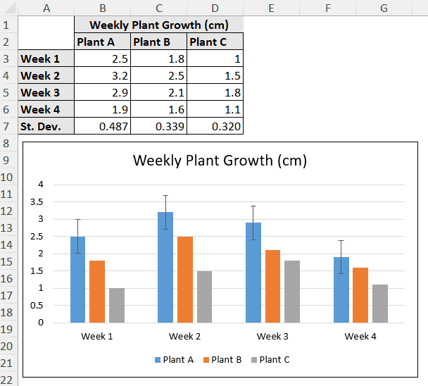
The series you have chosen before opening the Format Error Bars pane will now have individual error bars.
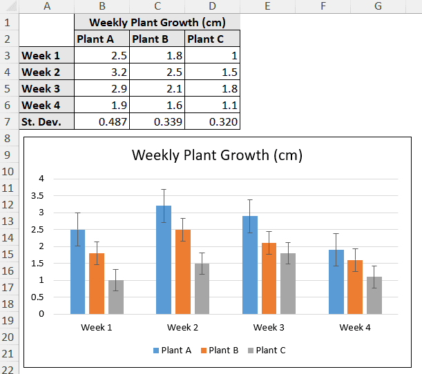
Step 5: Repeat for All Series (Optional)
In case you have multiple series, you need to repeat the process for all series individually to add the individual error bars.
We had multiple series for plants A, B, and C. So, we had to repeat it twice.
Let’s assume you only had two-dimensional data and a margin of error for each one. You could select the margin of error range directly in the positive and negative fields for the Custom Error Bars dialog box.
FAQ
How do I create custom error bars in Excel?
You can add fixed error bars, standard error bars, and standard deviation error bars directly from the Chart Elements button and the Chart Design tab.
To add more customization to an error bar, you need to select Custom from the Format Error Bars pane.
How can I remove individual error bars in Excel?
To remove an individual error bar, select the error bar individually before pressing Delete . You need to click on an error bar multiple times after selecting to select one individually.
Can I add separate positive and negative error bars for individual data points?
You can insert separate fields for positive and negative values in the Custom Error Bars dialog box after clicking on Specify Value. This will add separate positive and negative error bar values for a series or data point.
Why are my individual error bars not showing in Excel?
Error bars may not show because of formatting or values not being adjusted.
To avoid the problem of error bars not showing, make sure the error bars are correct colors to be visible. Then check if the positive or negative values are too little compared to the series values.
Conclusion
In this article, we have discussed how to add individual error bars in Excel. The key to adding an individual error bar is creating error bars for each series. To add a custom value, you need to use the Format Error Bars pane and insert values manually.
Feel free to download the practice workbook and give us your feedback.