Random sort in Excel means shuffling your data into a new order. Instead of sorting alphabetically or by numbers, Excel mixes up the rows so they appear in a completely random sequence.
This is helpful when you want to create random groups, pick winners for a draw, or just rearrange data without following any fixed rule.
Excel doesn’t have a direct random sort button, but you can do it easily using formulas like RAND or RANDBETWEEN, or by adding a helper column with random numbers.
In this article, you’ll learn simple methods to perform a random sort in Excel with three simple methods.
Here’s how to do a random sort in Excel using the RAND function:
➤ Open your dataset in Excel.
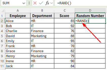
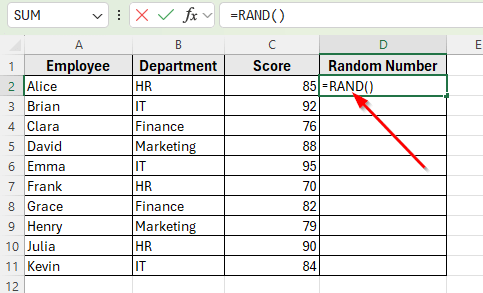
➤ In cell D2, enter the formula =RAND()
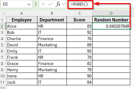
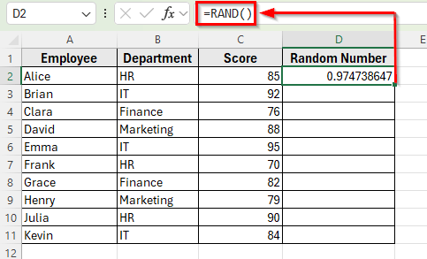
➤ Press Enter. You’ll see a random decimal number appear in the cell.
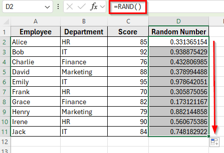
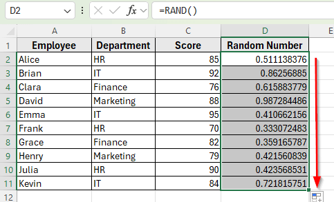
➤ Drag the fill handle down from D2 to D11 to fill random numbers for all employees.
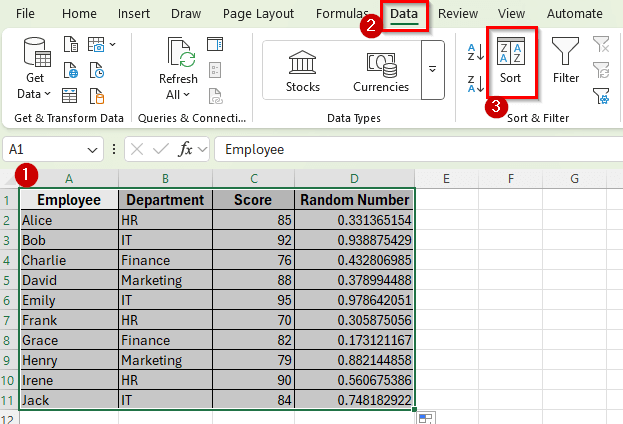
➤ Select the entire dataset, including the Random Number column.
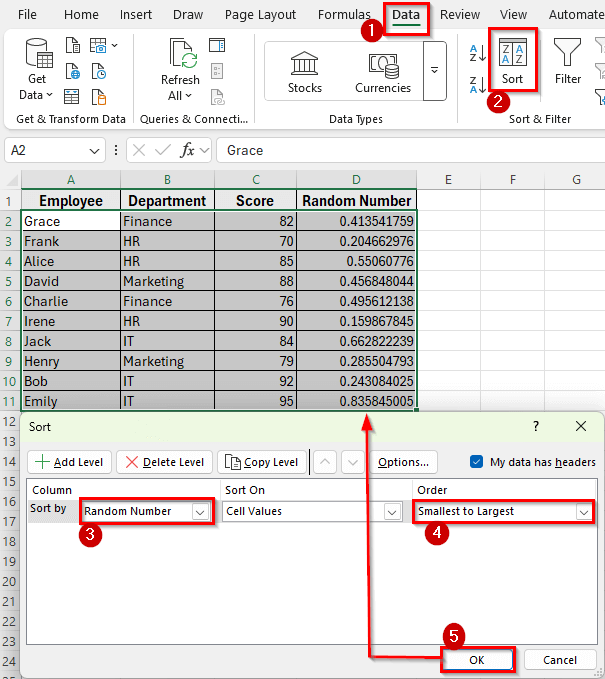
➤ Go to the Data tab on the ribbon, then click Sort.
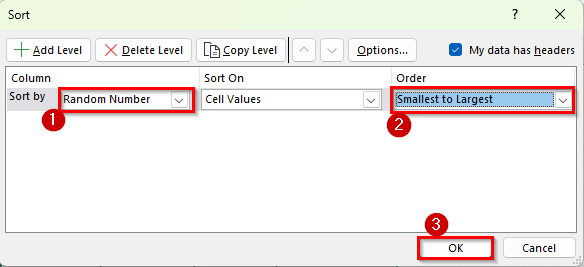
➤ In the Sort dialog box, choose Random Number as the column to Sort by. Select Smallest to Largest or Largest to Smallest in the Order box. It will not make any difference because the numbers are random.
➤ Click OK. Now the dataset will instantly rearrange into a random order.
Using the RAND Function for Random Sort in Excel
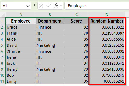
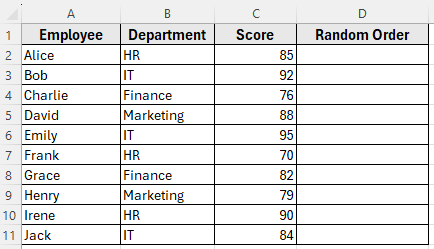
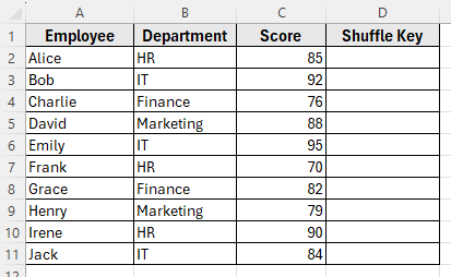
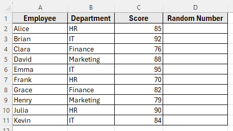
In the following dataset, we have a list of 10 employees along with their Departments and Performance Scores. Column A lists the Employee Names, Column B shows the Departments, and Column C contains their Scores.
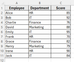
We’ll use this dataset to demonstrate how to shuffle rows randomly in Excel. Our goal is to randomly sort the employees so the order changes each time we apply a method.
The RAND function generates a random decimal number between 0 and 1. We can use it to create a helper column of random values, and then sort our dataset based on that column. This will shuffle the rows into a completely new order.
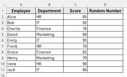
In this method, we’ll insert a new column next to your dataset and name it Random Number.
Here’s how to apply this method:
➤ Open your dataset in Excel.
➤ In cell D2, enter the formula
=RAND()
➤ Press Enter. You’ll see a random decimal number appear in the cell.
➤ Drag the fill handle down from D2 to D11 to fill random numbers for all employees.
➤ Select the entire dataset, including the Random Number column.
➤ Go to the Data tab on the ribbon, then click Sort.
➤ In the Sort dialog box, choose Random Number as the column to Sort by. Select Smallest to Largest or Largest to Smallest in the Order box. It will not make any difference because the numbers are random.
➤ Click OK.
➤ Now, the dataset will instantly rearrange into a random order.
Applying RANDBETWEEN Function for Random Sort in Excel
The RANDBETWEEN function generates random whole numbers between the two limits you specify. Unlike the RAND function, which produces decimals, this function returns integers. We can use those numbers as a helper column and then sort the dataset to shuffle the rows.
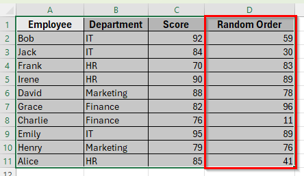
In this method, we’ll insert a new column next to your dataset and name it Random Order.
Here’s how to apply this method:
➤ Open your dataset in Excel.
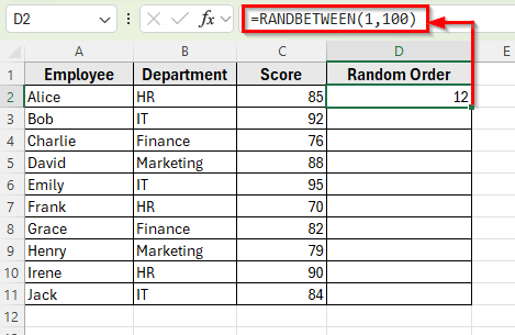
➤ In cell D2, enter the formula
=RANDBETWEEN(1,100)
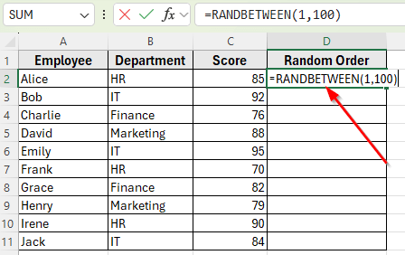
➤ Press Enter. Excel will return a random whole number between 1 and 100.
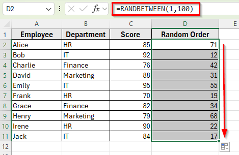
➤ Drag the fill handle down from D2 to D11 to fill numbers for all employees.
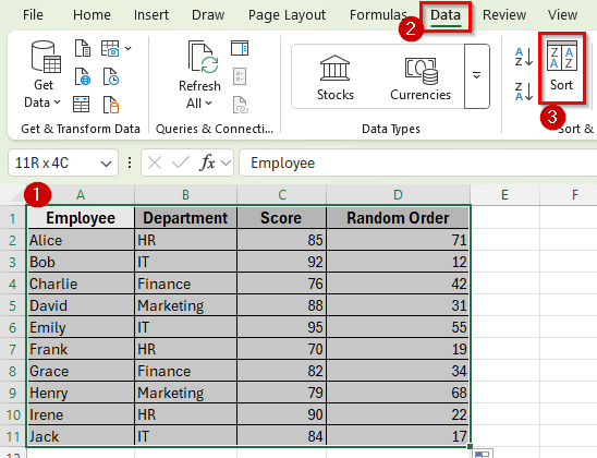
➤ Select the entire dataset, including the Random Order column.
➤ Go to the Data tab and click Sort.
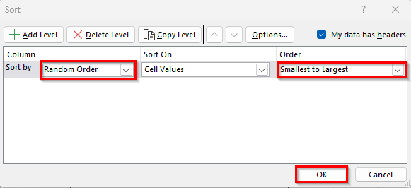
➤ From the Sort dialog box, choose Random Order as the column to Sort by. Select Smallest to Largest or Largest to Smallest in the Order box.
➤ Next, click OK.
➤ Now you’ll see the rows will now appear in a random sequence.
Using Manual Random Numbers for One-Time Shuffle
If you don’t want to use formulas, you can still create a random sort by manually typing numbers in a helper column and sorting the dataset by those numbers. This method gives you a one-time shuffle that won’t change when the worksheet recalculates.
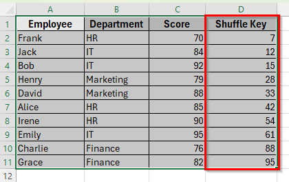
In this method, we’ll insert a new column next to your dataset and name it Shuffle Key.
Here’s how to do it:
➤ Open your dataset in Excel.
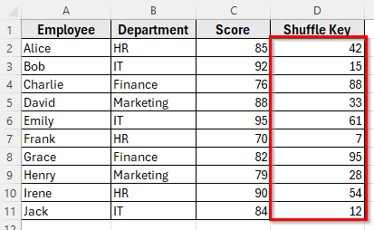
➤ In cells D2 to D11, type any random numbers in any order. For example:
42, 15, 88, 33, 61, 7, 95, 28, 54, 12
➤ Select the entire dataset, including the Shuffle Key column.
➤ Go to the Data tab on the ribbon and click Sort.
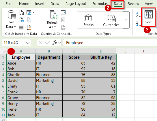
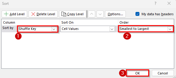
➤ A Sort dialog box will appear. Now select Shuffle Key as the column to Sort by. Select Smallest to Largest or Largest to Smallest in the Order box.
➤ Click OK.
➤ Your dataset will now be rearranged into a random order.
Shuffle Data with SORTBY, RANDARRAY, and ROWS Formula in Excel
If you are using Excel 365 or Excel 2021, you can combine the SORTBY, RANDARRAY, and ROWS functions to shuffle your dataset automatically. This is a formula-based method that does not require adding a helper column.
Here’s a simple step by step guide to apply this method:
➤ Open your dataset in Excel.
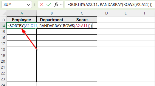
➤ Click on cell A14 where you want the shuffled result to appear.
➤ Enter the following formula:
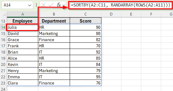
=SORTBY(A2:C11, RANDARRAY(ROWS(A2:A11)))
➤ Press Enter. Excel will instantly return the dataset in a new random order.
Apply RAND and SORT Functions Together for Random Sort
The SORT function can also be used to shuffle your dataset, but it works differently compared to SORTBY. With SORT, you need to specify the column number that Excel should use to sort the data. If that column contains random numbers which are generated by the RAND function, the dataset will be sorted randomly.
In this method, first, insert a helper column labeled Random Number in Column D.
Here’s how to do it:
➤ Open your dataset in Excel.
➤ In cell D2, type the formula
=RAND()
➤ Press Enter. You’ll see a random decimal number appear in the cell.
➤ Drag the fill handle down to fill random numbers for all rows.
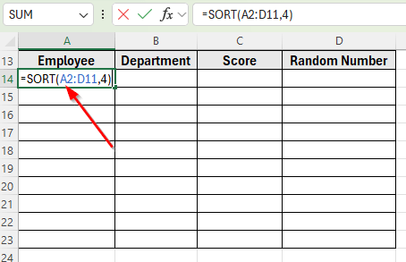
➤ Now, click on cell A14 and enter the following formula to sort the dataset randomly:
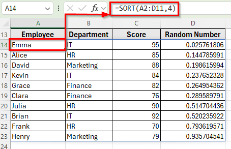
=SORT(A2:D11,4)
➤ Press Enter. Your dataset will appear in a new random order.
Using SORTBY with RANDARRAY and COUNTA for Random Sorting
Another dynamic way to shuffle data in Excel 365 or Excel 2021 is by combining the SORTBY, RANDARRAY, and COUNTA functions. This method works without a helper column and can randomize any dataset instantly.
Here’s how to apply this method:
➤ Open your dataset in Excel.
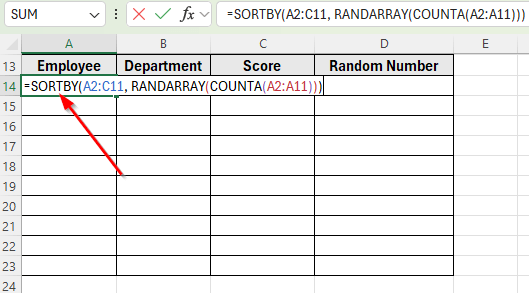
➤ Click on cell A14 where you want the randomized list to appear.
➤ Enter the following formula:
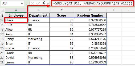
=SORTBY(A2:D11, RANDARRAY(COUNTA(A2:A11)))
➤ Press Enter. The dataset will now appear in a random order.
Apply VBA for Random Sorting in Excel
If you often need to randomize data, writing a simple VBA macro can save time. With VBA, you can shuffle your dataset instantly with just one click, without adding helper columns or formulas.
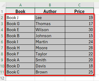
In this following dataset, here’s a list of books with their authors and prices. It contains three columns: Book in Column A, Author in Column B, and Price in Column C.
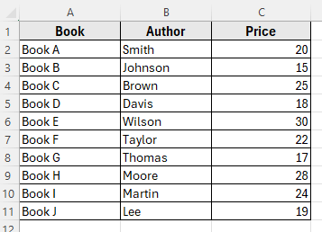
Our goal is to randomize the order of these rows using a VBA macro. This way, each time we run the macro, the books will appear in a different order.
Here’s how to apply VBA for random sorting:
➤ Open your dataset in Excel.
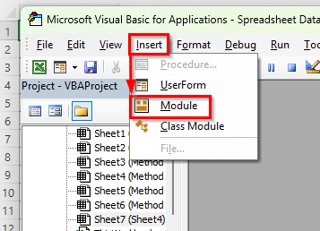
➤ Press Alt + F11 to open the VBA editor.
➤ In the VBA window, click Insert >> Module.
➤ Copy and paste the following code into the module:
Sub Random_Sort()
    Dim rng As Range
    Dim cell As Range
    'Select the dataset range
    Set rng = Selection
    'Add a helper column with random numbers
    rng.Offset(0, rng.Columns.Count).Resize(rng.Rows.Count, 1).Formula = "=RAND()"
    'Sort based on the random numbers
    rng.Resize(rng.Rows.Count, rng.Columns.Count + 1).Sort _
        Key1:=rng.Offset(0, rng.Columns.Count), Order1:=xlAscending, Header:=xlNo
    'Remove helper column
    rng.Offset(0, rng.Columns.Count).Resize(rng.Rows.Count, 1).ClearContents
End Sub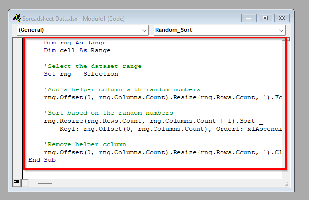
➤ Close the VBA editor and return to Excel.
➤ Select the range of your data like A2:C11.
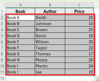
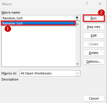
➤ Press Alt + F8 , choose Random_Sort, and click Run.
➤ Your dataset will be randomized instantly.
Frequently Asked Questions
How to randomly sort data in Excel?
You can insert a helper column with random numbers and then sort your dataset by that column. The easiest way is to use the RAND function, fill it down for all rows, and then sort the data based on those values.
What is the formula for random sort?
The most common formulas for random sorting are =RAND() and =RANDBETWEEN(1,100). The RAND function returns decimal numbers between 0 and 1, while the RANDBETWEEN function returns whole numbers between the limits you set. Sorting by either column will shuffle your rows randomly.
How do I keep the random order fixed?
If you want to lock the random order so it doesn’t change, copy the helper column with random numbers and paste it back as values. This prevents Excel from recalculating the random numbers and keeps your dataset in the same order.
Wrapping Up
Random sort in Excel is a quick way to shuffle rows when you don’t want them in a fixed order. You can use functions like RAND or RANDBETWEEN to create a helper column and then sort the dataset, or you can type random numbers manually for a one-time shuffle.
Each method works for different needs. If you want the ability to reshuffle anytime, RAND and RANDBETWEEN functions are the best options. If you want the random order to stay fixed, using manual numbers or pasting random values works better.
With these techniques, you can easily randomize your data for tasks like assigning teams, drawing winners, or preparing samples in Excel.