Sorting is one of the most common tasks in Excel. Normally, you select your data and use the Sort button to organize it. But what if your dataset changes frequently?
For example, when new entries are added or existing values are updated, you don’t want to manually sort it every time. Instead, you can set up auto sort so Excel automatically keeps your list organized.
There are many different ways to make Excel auto sort your data. In this article, you’ll learn how to auto sort in Excel when data changes using formulas and VBA.
Here’s how to auto sort data in Excel when values change:
➤ Open your dataset in Excel.
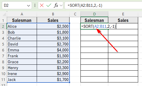
➤ Click on cell D2, where you want the sorted result to appear.
➤ Enter the following formula:
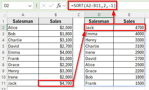
=SORT(A2:B11,2,-1)
➤ Press Enter. You’ll now see a new table with sales values arranged from largest to smallest.
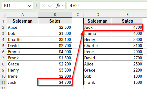
➤ Now, change Jack’s sales from $1,700 to $4,700, that’ll place Jack at the top of the list.
Apply SORT Function to Auto Sort in Order When Data Changes
In this following dataset, we have a list of Salesmen and their Sales values. Column A labeled Salesman and Column B labeled Sales values. In Column D and E, we’ll make a second table where we’ll apply different formulas to demonstrate auto sort in Excel.
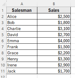
We’ll use this dataset to make this table automatically re-sort itself whenever the Sales values are updated.
The SORT function is the simplest way to make Excel automatically sort your data when values change. It allows you to define a range, choose the column to sort by, and specify whether you want ascending or descending order. Whenever you update the original dataset, the sorted table updates instantly.
The generic formula is
=SORT(array, [sort_index], [sort_order], [by_col])
Auto Sort in Descending Order
In this method, we want to display the sales in descending order, from the highest to the lowest.
Here’s how to apply this method:
➤ Open your dataset in Excel.
➤ Click on cell D2, where you want the sorted result to appear.
➤ Enter the following formula:
=SORT(A2:B11,2,-1)
➤ Press Enter. You’ll now see a new table with sales values arranged from largest to smallest.
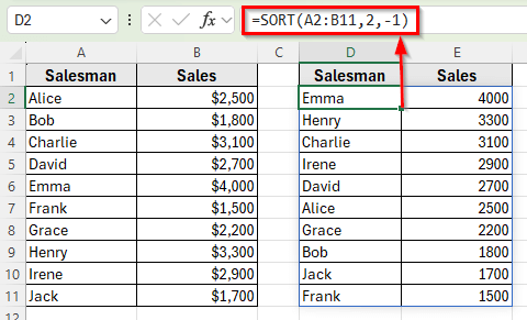
➤ Now, change Jack’s sales from $1,700 to $4,700, that’ll place Jack at the top of the list.
Auto Sort in Ascending Order
In this method, we want to display the sales in ascending order, from the lowest to the highest.
➤ Click on cell D2, where you want the sorted result to appear.
➤ Enter the following formula:
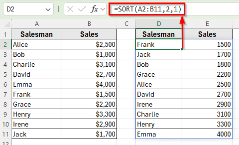
=SORT(A2:B11,2,1)
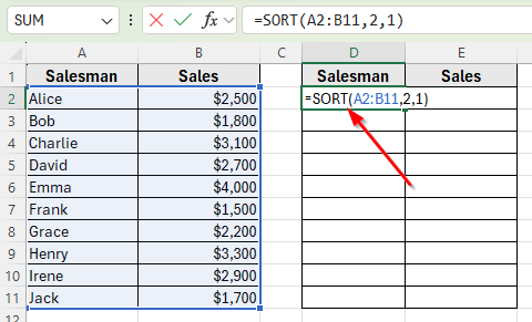
➤ Press Enter. The new table will appear with the Sales values sorted from the smallest to the largest.
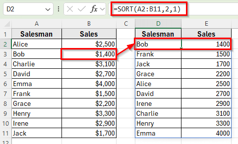
➤ Now, change the sales value of Bob from $1,800 to $1,400, the sorted row will automatically rearrange in ascending order and place Bob at the top of the list.
Auto Sort Multiple Columns with Different Orders
Sometimes you may need to sort a table by more than one column, each in a different order. For example, you might want to sort first by a Counter column in ascending order and then by Sales in descending order. Excel’s SORT function can handle this easily.
In this method, add a Counter column in the middle of the Salesman and Sales value column.
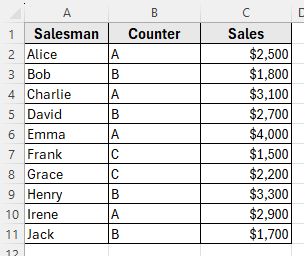
Our goal is to sort this table so that the Counter column is in ascending order like A >> B >> C, while the Sales column is in descending order within each counter group.
Here’s how to do it:
➤ Click on cell E2, where you want the sorted table to appear.
➤ Enter the following formula:
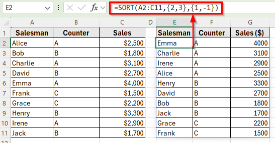
=SORT(A2:C11,{2,3},{1,-1})
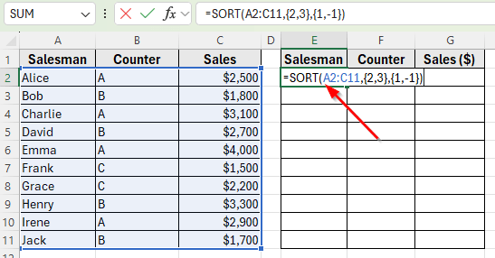
➤ Press Enter. The table will now sort first by Counter in ascending order, and then by Sales in descending order for each group.
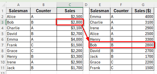
➤ Now, change Bob’s sales value from $1,800 to $2,800, the sorted table will update automatically and place Bob in the correct position within the B group.
Apply SORT Function to Auto Sort by Columns
The SORT function allows you to sort data horizontally by specifying the column sorting argument.
In this following dataset, we’ll transpose the table so that the Salesmen are listed in Row 1 and their corresponding sales are in Row 2.
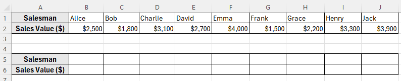
Our goal is to sort the sales in descending order across the row.
Here’s how to do it:
➤ Select cell B5, where you want the sorted row to appear.
➤ Enter the following formula:
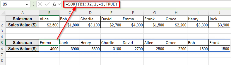
=SORT(B1:J2,2,-1,TRUE)
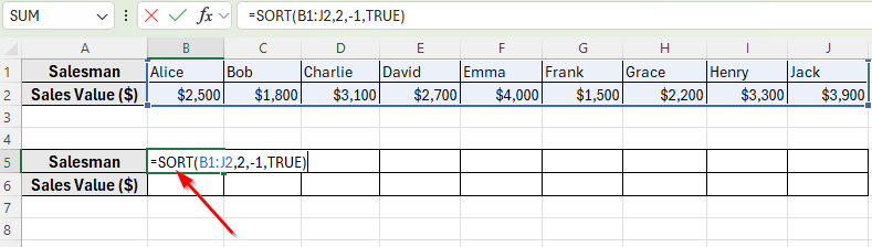
➤ Press Enter. The table will now display the Sales values in descending order from left to right.
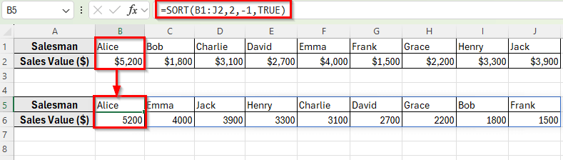
➤ Next, update Alice’s sales from $2,500 to $5,200, the sorted row will automatically rearrange to reflect the new order.
Use SORT with FILTER to Auto Sort by Conditions
You can combine the FILTER and SORT functions to sort only a specific subset of your data instead of the entire table.
In this method, we’ll filter only the Sales values greater than $2,500 and then auto sort them in descending order.
Here’s how to do it:
➤ Click on cell D2, where you want the filtered and sorted output.
➤ Enter the following formula:
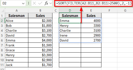
=SORT(FILTER(A2:B11,B2:B11>2500),2,-1)
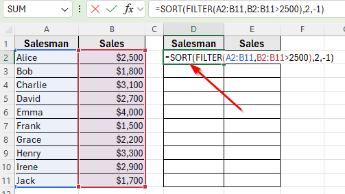
➤ Press Enter. You will now see only the rows where Sales are greater than $2,500, sorted from the highest to the lowest.
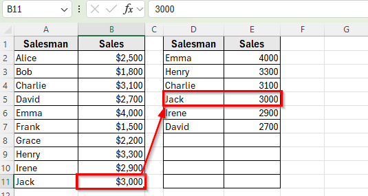
➤ Next, update any sales value in the original row. For example, change Jack’s sales from $1,700 to $3,000, the sorted row will automatically rearrange to reflect the new order.
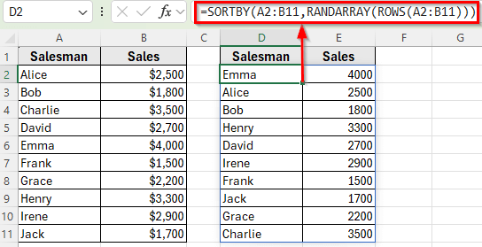
Apply SORTBY with RANDARRAY to Auto Sort Randomly
There may be situations where you don’t want to sort your data in ascending or descending order but instead need to shuffle the rows randomly.
In this method, our goal is to randomly shuffle this table so that the order changes every time the worksheet recalculates.
Here’s how to do it:
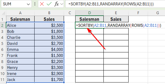
➤ Click on cell D2, where you want the randomized list to appear.
➤ Enter the following formula:
=SORTBY(A2:B11,RANDARRAY(ROWS(A2:B11)))
➤ Press Enter. The dataset will now appear in a random order.
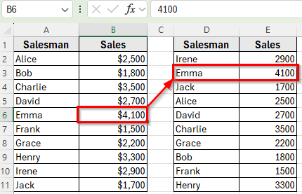
➤ Now, change Emma’s sales from $4,000 to $4,100, the sorted row will automatically rearrange to reflect the new order.
Extracting Highest or Lowest 3 Values Based on Data Update By Sorting
Sometimes you don’t need the entire dataset sorted, but only want to display the top performers. By combining the INDEX, SORT, and SEQUENCE functions, you can automatically extract the top 3 highest and lowest sales values and their corresponding salesmen.
Here’s how to apply this method:
Auto Sort the Top 3 Highest Values
In this method, our goal is to display only the top 3 highest sales values in descending order.
➤ Click on cell D2, where you want the top 3 highest sales list to appear.
➤ Enter the following formula:
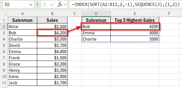
=INDEX(SORT(A2:B11,2,-1),SEQUENCE(3),{1,2})
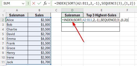
➤ Press Enter. The new table will now show the top 3 salesmen with their sales values.
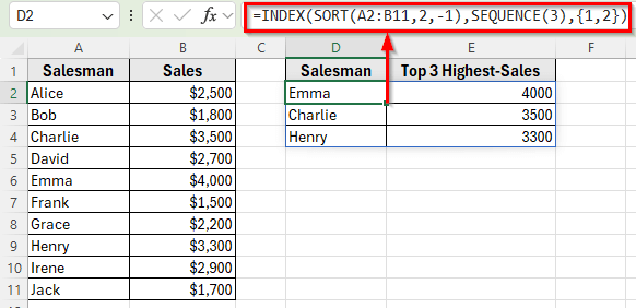
➤ Now, updating Bob’s sales from $1,800 to $4,200, Bob will move into the top 3 automatically.
Auto Sort the Top 3 Lowest Values
In this method, our goal is to extract the top 3 lowest sales values in ascending order.
➤ Click on cell D2, where you want the top 3 lowest sales list to appear.
➤ Enter the following formula:
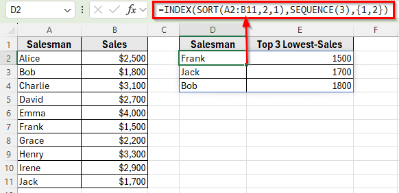
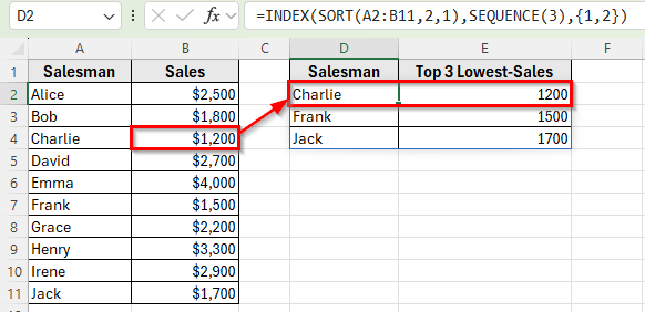
=INDEX(SORT(A2:B11,2,1),SEQUENCE(3),{1,2})
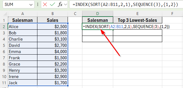
➤ Press Enter. The table will now display the 3 lowest sales values in ascending order.
➤ Next, update Charlie’s sales from $3,100 to $1,200, Charlie will appear in the top 3 lowest sales list instantly.
Use INDEX and SORT to Auto Extract a Specific Ranked Value
Sometimes you may want to pull only a particular ranked value, such as the second-highest or second-lowest sales figure, instead of sorting the entire table. By combining the INDEX and SORT functions, you can do this dynamically without needing helper columns.
Get the Second-Highest Value
➤ Click on cell D2 and enter the following formula:
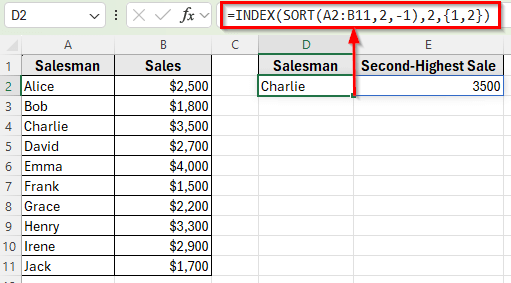
=INDEX(SORT(A2:B11,2,-1),2,{1,2})
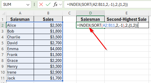
➤ Press Enter. The formula will return the second-highest sales record, including the Salesman’s name and Sales figure.
Get the Second-Lowest Value
➤ Click on cell D5 and enter this formula:
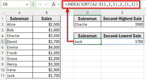
=INDEX(SORT(A2:B11,2,1),2,{1,2})
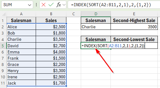
➤ Press Enter. This will return the second-lowest sales record dynamically.
➤ Now, whenever you update any Sales figure in the original dataset, the extracted second-highest or second-lowest record will update instantly.
Auto Sort While Adding New Rows to the Table
Until now, the methods worked when changing values, but not when adding new rows. To fix this, turn your dataset into an Excel Table. This way, the sorted list will update automatically whenever you add a new Salesman and Sales value.
Here’s how to apply this method:
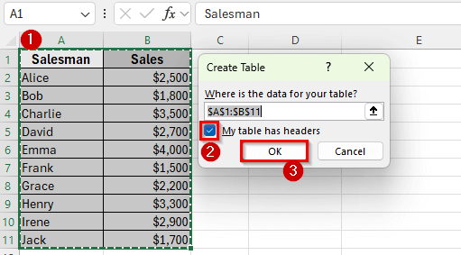
➤ Select the dataset range A2:B11.
➤ Press Ctrl + T to convert the dataset into a Table format. Make sure the option My table has headers is checked.
➤ Now click on cell D2 and enter the following formula:
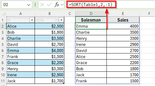
=SORT(Table1,2,-1)
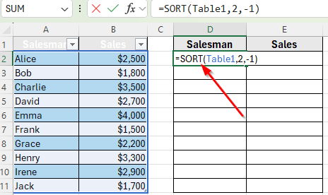
➤ Press Enter. The sorted table will appear with the Sales figures arranged in descending order.
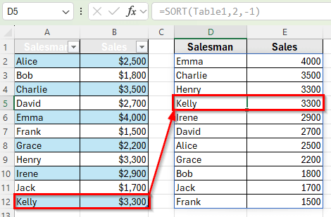
➤ Next, type a new record below the original dataset, for example: Salesman Name: Kelly and Sales value $3,300.
➤ The sorted table will immediately include the new record and rearrange the order based on the updated Sales values.
Auto Sort with VBA Macro (For All Excel Versions)
If you prefer automation beyond formulas, you can use VBA to make Excel auto sort the dataset whenever changes occur.
In this method, we’ll write a small VBA script to automatically sort the table whenever the Sales values are updated or new rows are added.
Here’s a simple step-by-step guide how to apply this method:
➤ Press Alt + F11 to open the VBA Editor in Excel.
➤ In the VBA window, double-click on the worksheet name under your workbook. For example, Sheet11.
➤ Copy and paste the following VBA code:
Private Sub Worksheet_Change(ByVal Target As Range)
    ' Check if the change happens in column B (Sales column)
    If Not Intersect(Target, Me.Range("B2:B11")) Is Nothing Then
        ' Disable events to prevent looping
        Application.EnableEvents = False
        ' Sort the range A2:B11 based on Sales column in descending order
        Me.Range("A1:B11").Sort Key1:=Me.Range("B2"), _
        Order1:=xlDescending, Header:=xlYes
        ' Enable events again
        Application.EnableEvents = True
    End If
End Sub 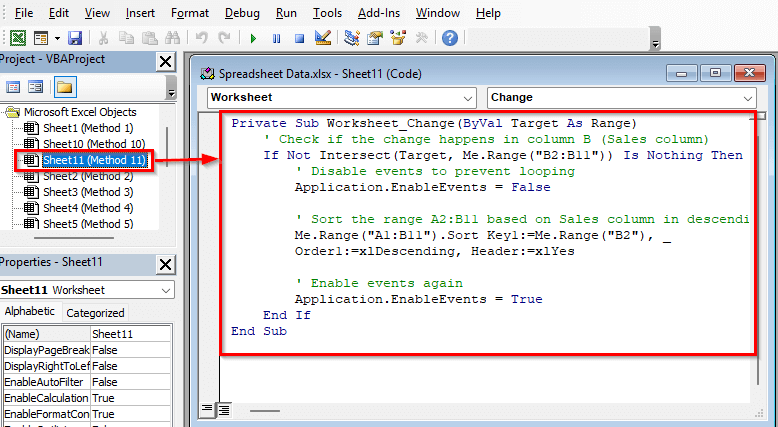
➤ Close the VBA editor and return to Excel.
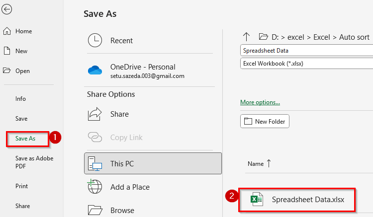
➤ Save the file as a Spreadsheet Data.xlsx.
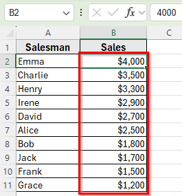
➤ Now, in column B, the Sales values appear in descending order.
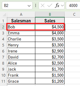
➤ Now, update Bob’s sales from $1,800 to $4,500, the dataset will instantly rearrange and place Bob at the top of the list without you pressing any buttons.
Frequently Asked Questions
How do I make Excel auto SORT when data changes?
You can use the SORT function with a dynamic range or convert your dataset into an Excel Table. This way, whenever you update a value, the sorted output will refresh automatically. For full automation, you can also apply a VBA macro that sorts the data every time a change is made.
How do I SORT data dynamically in Excel?
Dynamic sorting is possible with functions like SORT, FILTER, SEQUENCE, and INDEX. For example, the formula =SORT(B5:C14,2,-1) will always sort your dataset by the second column in descending order. Any time you update the source data, the sorted results update automatically.
Does Excel have auto SORT?
Yes. While Excel does not have a direct Auto Sort button, you can achieve auto sorting by using formulas like SORT or FILTER, converting your data into a Table, or by applying a simple VBA script. These methods ensure your data rearranges itself without needing manual sorting.
Wrapping Up
Auto sorting in Excel saves time and keeps your data organized without repeated manual steps. Depending on your needs, you can use formulas like SORT, FILTER, INDEX, and SEQUENCE, or even apply VBA for complete automation.
Choose the method that fits your workflow best. Once set up, Excel will do the sorting work for you, so you can focus on analyzing the results instead of managing the order of your data.