How to Create a Table in Excel from Existing Data​

Excel tables are structured ranges of data with added functionality, such as automatic column headers, built-in filtering and sorting, and predefined styles/formatting. They make managing, analyzing, and formatting data much easier.

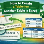
Excel allows you to readily convert your existing dataset into a table. Whether it’s a range or data from a single cell, you can convert any data into a table in just a few clicks.

Our sample dataset has 4 columns for product codes, salesperson’s names, product names, and prices. We’ll turn the entire range A1:D10 into a table.

On your Excel’s main ribbon, the Insert tab has the Table option, which allows you to insert a new table and convert a range into a table. Here’s how:

➤ Click on any cell of your data range. Go to the Insert tab and click on Table from the Tables group.

➤ Now, Excel will open the Create Table box. It automatically selects your entire data range. Edit the range if you want. If your data has column headings, keep the My Table Has Headers box checked. Otherwise, you can uncheck it. Click Ok.

➤ Your data range is now a table. Click on any cell of the table and use the Table Design tab to style and format your table. Consider the following options:

• Table Name: In the Table Design tab, go to the Properties group, and enter a name (without any spaces) in the Table Name Press Enter.

• Alternate Shading: The Table Styles group in the Table Design tab has many alternate shading colors. Click on any of them to apply one.

• Sort or Filter Data: Click on the drop-down on any column header and select any sorting or filtering option you prefer. Press Ok.

• Add Total Row: From the Table Style Options group (Table Design tab), check the Total Row box to sum any column containing numbers. You can also uncheck the Filter Button box here to remove the filter drop-downs from the table headers.

Follow the steps given below to instantly turn a data range into a table:

➤ Select any cell in the range and press  Ctrl  +  T  on your keyboard.
➤ In the Create Table box, choose the range to convert and check the My Table Has Headers box as needed. Click Ok.

➤ Customize table styles using the Table Design tab.

With the Power Query tool, you can turn existing data into a table, transform or edit it, and load it in the same or different worksheet. Below are the steps:

➤ Right-click on any cell within the range and choose From Table/Range from the menu.

➤ As Excel prompts you to confirm the range, select your range, confirm headers, and click Ok.

➤ Your data will open in the Power Query Editor.

➤ Use the different tabs in Power Query to remove blank rows/columns, change column data types, split/merge columns, filter records, etc.
➤ For example, we’ll split the names in Column B into two different columns. First, click on the column, open the Transform tab and press the Split Column drop-down.
➤ As our data is separated by a space, we selected By Delimiter. Choose the right option according to your dataset.

➤ In the new dialog box, select the correct delimiter (e.g., Space) and press Ok.

➤ Excel will now split the column into two.

➤ Click on the column headers to edit the name of each column. Once the editing is done, go to the Home tab >> Close & Load drop-down >> Close & Load To…

➤ In the Import Data dialog box, choose Table and select where to place it (New Worksheet or Existing Worksheet). Click Ok.

➤ Here’s the final result:

The Text to Columns Wizard helps you split text data into structured columns and then convert it into a table. We have entered the necessary data for the table in Column A (separated by comma). First, we’ll place the texts in separate columns and then turn the range into a table. Here’s how:

➤ Select the column containing the text data. Go to the Data tab and click on Text to Columns in the Data Tools group.
➤ In Step 1 of the Convert Text to Columns Wizard, select Delimited if your data uses commas, tabs, or other separators). Or, choose Fixed Width if the columns are aligned with spaces. Click Next.

➤ From Step 2, you can choose the type of delimiter your data is separated by. We selected Comma. Press Finish.

➤ Now, the data is split into proper columns.

➤ Format the headers, and data type as needed. Finally, select a cell and use Insert >> Table or  Ctrl  +  T  to turn it into a formatted Excel table.

If you frequently create tables, you can automate the process with a VBA macro. Let’s get to the steps:

➤ Click on the sheet name and select View Code from the menu.

➤ In the blank field, copy and paste the following code:

Sub CreateTableFromRange()
    Dim rng As Range
    Dim tbl As ListObject
    Dim ws As Worksheet
    Dim tblName As String
    'Set the worksheet
    Set ws = ActiveSheet
    'Prompt user to select a range
    On Error Resume Next
    Set rng = Application.InputBox("Select the range you want to convert into a Table:", _
                                   "Select Range", Type:=8)
    On Error GoTo 0
    'Exit if no range is selected
    If rng Is Nothing Then
        MsgBox "No range selected. Operation cancelled.", vbExclamation
        Exit Sub
    End If
    'Ask user for a table name
    tblName = Application.InputBox("Enter a name for your Table:", "Table Name", "MyTable")
    If tblName = "" Then tblName = "MyTable"
    'Check if the table name already exists
    On Error Resume Next
    Set tbl = ws.ListObjects(tblName)
    On Error GoTo 0
    If Not tbl Is Nothing Then
        MsgBox "A table with this name already exists. Please try again with a different name.", vbCritical
        Exit Sub
    End If
    'Convert the selected range into a Table
    Set tbl = ws.ListObjects.Add(xlSrcRange, rng, , xlYes)
    tbl.Name = tblName
    'Apply a built-in Table Style
    tbl.TableStyle = "TableStyleMedium9"
    MsgBox "Your selected range has been successfully converted into a Table named '" & tblName & "'.", vbInformation
End Sub

➤ Press  F5  on your keyboard or go to the Run tab >> Run Sub/UserForm.

➤ When the Select Range dialog box opens, go back to the Excel tab and choose the range you want to convert. Press Ok.

➤ Give your table a name in the Table Name box. Click Ok.

➤ Your range is now converted. Use the Table Design tab to customize it.

Frequently Asked Questions

How to revert an Excel table to a range?

Click on any cell of your table and go to the Table Design tab. Expand the Table Styles section and press Clear to remove table formatting. From the Tools group, click on the Convert to Range option.

How do I resize the table in Excel?

Click anywhere inside the table and go to the Table Design tab. In the Properties group, click on the Resize Table option. As a dialog box appears, select the new range of cells you want the table to cover and click Ok.

How do I remove duplicates in an Excel table?

Select a table cell and go to the Data tab. Click Remove Duplicates in the Data Tools group. Select the columns where you want to check for duplicates. Click Ok, and Excel will remove the duplicate values, keeping only the first occurrence.

Concluding Words

Choose the correct method of creating a table based on your dataset. Although you can’t directly convert non-adjacent columns into a table, you can load your data in Power Query and select only the columns you want (even if they’re non-adjacent). Every time you add new columns or rows right next to your table, it will expand automatically.