Large numbers, such as sales or revenue data, can be overwhelming in raw form. Instead of reading values like 5,870,000, you can make your spreadsheets more readable by displaying them as 5.9 M. Excel’s custom number formatting and related tools let you format values in millions with one decimal place, improving clarity and saving space in reports or dashboards.
If your dataset contains a mix of values like- some in the thousands and some in the millions, then you may also want to explore formatting numbers with K for thousands and M for millions so that all figures are scaled appropriately in the same column.
In this article, you’ll learn six effective techniques for formatting numbers as millions with one decimal in Excel. Whether you prefer custom formats, formulas, or conditional formatting, these methods will make your worksheets cleaner and easier to interpret.
Steps to use custom number format millions with one decimal in Excel:
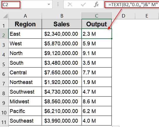
➤ In C2, type: =TEXT(B2,”0.0,,”)&” M”
➤ Drag down to C11.
➤ This produces a string like 3.5 M, which won’t affect calculations but is great for labels or dashboards.

Apply a Basic Custom Format with Zero Placeholder
When you need a quick and reliable way to show numbers in millions with one decimal, using a custom number format with the zero placeholder is one of the simplest options. The zero (0) ensures that even numbers without a fractional component display a digit, creating a uniform look across your data. This is especially helpful for financial reports or dashboards where consistency matters.
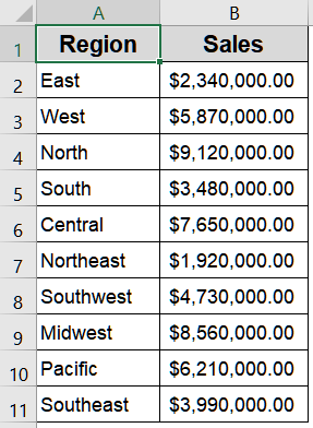
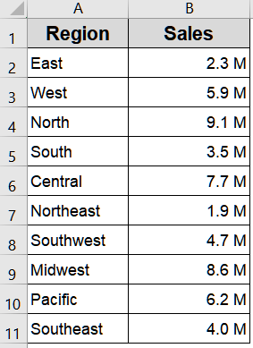
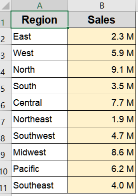
We’ll use the following dataset:
Steps:
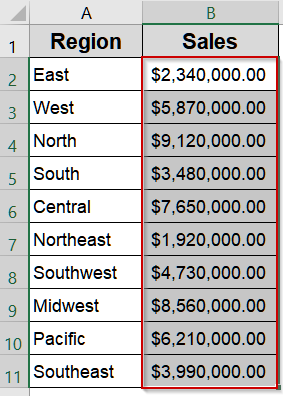
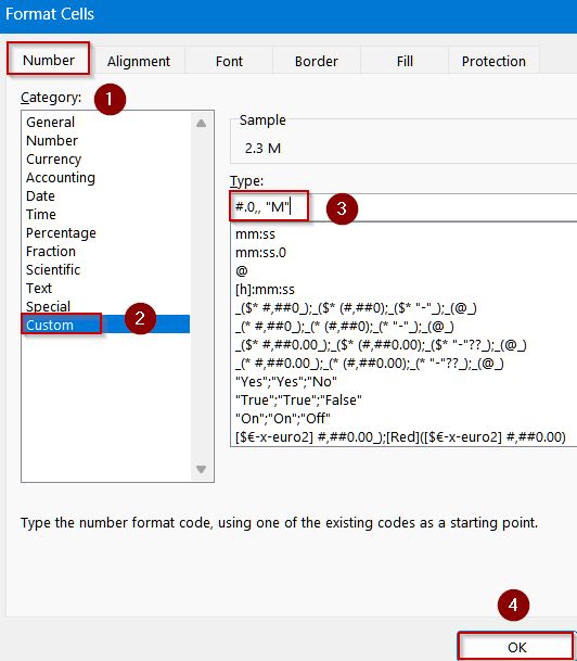
➤ Select the range B2:B11 containing your sales data.
➤ Press Ctrl + 1 (or right-click and choose Format Cells).
➤ In the Number tab, go to Custom.
➤ Type this formula: 0.0,, “M”
➤ Click OK.

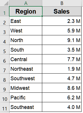
➤ Your numbers will now display like 5.9 M while retaining their full values for calculations.
The “M” suffix here is embedded directly in the format code. If you want to learn more about adding any custom text or unit label after a number, our article on how to add text after a number using a custom format covers the full technique in detail.
Use a Flexible Hashtag Symbol for Cleaner Formatting
For those who want a slightly sleeker look, the hashtag (#) symbol is perfect. Unlike zero placeholders, hashtags suppress unnecessary leading or trailing zeros, making your dataset appear cleaner and more polished. This is ideal when you’re working with values that vary in length, as it prevents awkward extra zeros from appearing.
Steps:
➤ Highlight the same sales values in B2:B11.

➤ Open Format Cells using Ctrl + 1 .
➤ Under Custom, type: #.0,, “M”
➤ Press OK and notice values like 7.7 M or 9.1 M displayed neatly without extra zeros.
Round Values with a Formula Before Appending "M"
Sometimes, you may want more control over rounding or to display formatted numbers in a separate column, leaving your original data unchanged. Using the ROUND function makes this easy by converting numbers to millions and appending “M” directly in a new column. We’ll also use the Paste Special feature to modify the original column permanently.
Steps:
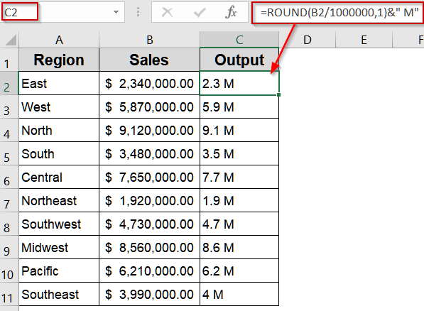
➤ In cell C2, enter:
=ROUND(B2/1000000,1)&" M"
➤ Drag the formula down through C11.
➤ The results will show 2.3 M, 5.9 M, etc., rounded to one decimal place.
➤ Copy the range C2:C11.
➤ Right-click on B2 and choose Paste Values under Paste Options.
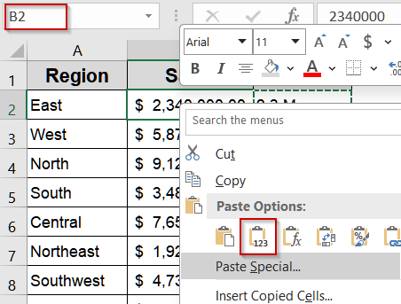
➤ Delete column C. Your original column B now permanently displays millions with one decimal.

Use the TEXT Function for Full Control Over Appearance
When you need both flexibility and precision in displaying values, the TEXT function is your best choice. Unlike basic number formats, TEXT function allows you to convert a number into a formatted string in a single step. This is especially useful for dashboards, reports, or when concatenating labels with other text. By using this function, you can display numbers exactly how you want such as millions with one decimal without altering the original values stored in your worksheet.
Steps:
➤ In C2, type:
=TEXT(B2,"0.0,,")&" M"
➤ Drag down to C11.
➤ This produces a string like 3.5 M, which won’t affect calculations but is great for labels or dashboards.
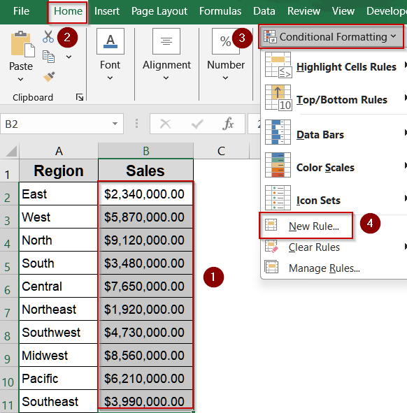
Highlight Values Dynamically with Conditional Formatting
If you want your large numbers to stand out visually while also showing them in millions, conditional formatting provides a dynamic and automated solution. This method is perfect when working with large datasets or dashboards where certain thresholds need emphasis. By combining custom number formatting with conditional rules, you can apply distinct formats only when values meet specific conditions, like highlighting all sales figures above one million.
Steps:
➤ Select B2:B11.
➤ Go to Home >> Conditional Formatting >> New Rule.
➤ Choose Format only cells that contain, set the condition (e.g., Cell Value ≥ 1000000).
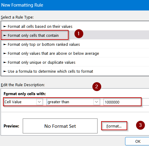
➤ Click Format >> Number >> Custom and enter: 0.0,, “M”
➤ Apply a fill or font color if desired, then click OK.
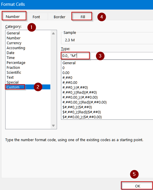
➤ Large values now display as millions with one decimal and are highlighted for better visibility.
Or If you want to go further and apply different number formats based on value thresholds, such as- showing one format for values above a million and another for values below, then check out our article on custom number formats with multiple conditions in Excel.
Frequently Asked Questions
Can I still perform calculations on numbers formatted as millions?
Yes. Custom number formats only change how values are displayed, not their underlying values. You can continue to use these numbers in formulas, charts, and summaries without affecting calculations.
Will using the TEXT function affect numeric calculations?
Yes. The TEXT function converts numbers into text strings. While it’s useful for labels or reports, you can’t directly perform numeric calculations on TEXT results unless you convert them back to numbers.
Will my values smaller than a million show as “M”?
Values below one million will display as decimals smaller than 1 such as 0.8 M for 800,000. For such cases, consider adding conditions or alternative formats to improve clarity in your worksheet.
Can conditional formatting automatically update when values change?
Yes. Conditional formatting dynamically reacts to changes in your data. If you update or replace values, Excel will immediately reapply the custom number format and any highlighting based on your specified rules.
Do custom formats work in charts or pivot tables?
Yes. If the underlying cell values are formatted, charts and pivot tables will also display numbers using the custom million format. This ensures consistency and readability across your reports and visualizations.
Wrapping Up
Formatting values as millions with one decimal in Excel keeps your spreadsheets concise and professional. Whether you use custom formats, formulas, or conditional formatting, these methods help you present large numbers clearly without altering their underlying values. By practicing these techniques with the provided dataset, you can quickly upgrade your dashboards and reports for improved readability and impact.