Column headers in Excel are the titles you see at the top of each column. They play a vital role in data management. These headers help you and others understand what kind of data is stored in each column.
No one will understand what’s the data about or where’s the required data in the dataset by just seeing Column A or Column B or even sometimes nothing at all there. So, column headings act like just street signs, guiding you throughout the datasets. So, it’s crucial to create column headers in excel.
Fortunately there are more than one ways with several purposes to make a column heading. In this article, we’re going to learn some of the most effective ways to add column headers in excel. Firstly, here’s a straightforward approach to get started.
➤ Firstly, insert a new blank row in row 1.
➤ Then convert the data into a table by choosing Format as table.
➤ Once the column headers are created, type the headings as required.
Now let’s dive into the details. We’ll explore multiple methods to add column headers in excel.
Creating Column Headers Manually in Excel
The most straightforward way to create column headings in an excel dataset is adding the headers manually. To do so, we just type the header text directly into the cells of the first row. This would be the simplest but it is not likely to be a structured approach especially for larger datasets.
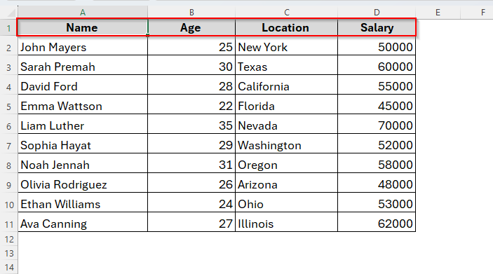
However, here we have an example dataset including four different columns without column headers. So, it seems so confusing about what kind of data these columns have.
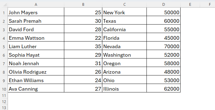
To solve this, we’ll attach column headers manually in this dataset and below we discuss how it goes.
Steps:
➤ Firstly, open the worksheet where you want to create the column headers.
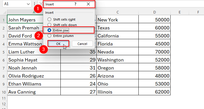
➤ Now we have to insert a blank row as there’s no blank cells where we could type the header text. So, right click on cell A1 and choose Insert. Then, select Enter Row and tap Ok.
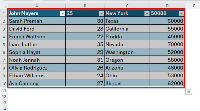
➤ Next, in the first row where you want the headings, type the title of each column and modify the cell color, font, and position as the image shows below.
Note:
Press Tab to move to the next column and continue the process for each column you want to cover.
Using Freezing Panes Option to Make Column Headers Remaining Visible
Sometimes when we scroll down to our dataset, the headers disappear. As a result, we may lose track or could get confused about what the columns show.
Let’s assume you’re scrolling down a giant Excel sheet with 5,000 rows. By row 50, the headers have vanished, and you’re left guessing what column D was supposed to mean. Frustrating, right? In this case, freezing panes allows headers to remain visible even when we scroll down.
Steps:
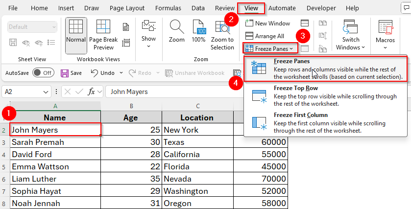
➤ Click on the row just below the headings like here we selected cell A2.
➤ Then go to the View tab.
➤ Now choose the Freeze Panes option. Here we’ll get a list of three different freezing options. From there, just select Freeze Panes.
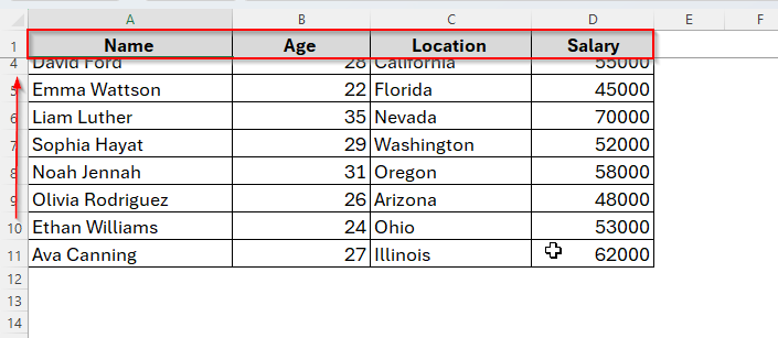
➤ Now if we scroll down to the sheet as you can see in the following image, the headers don’t disappear. They have been frozen and we can easily locate the heading for each column.
Note:
If your column headers are in row 1, then you can also choose the Freeze Top Row option. But if the headings are in different rows like 3,4 or 5, then click on Freeze Panes. It will lock the row above the one you clicked in the beginning.
Creating Column Headers by Formatting as a Table
By default, Excel inserts column headers automatically in tables. So, if we turn our data into a table, it will add automatic headers. To convert your data into a table, below are the steps to follow.
Steps:
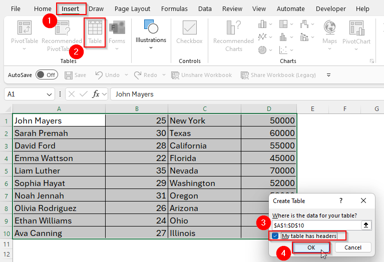
➤ Select the data range from A1 to D10.
➤ Go to the Insert → Table.
➤ Ensure My table has headers option checked and tap Ok.
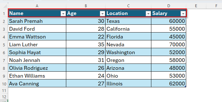
➤ Once you click Ok, the table has been created as follows including a header row.
Now the headers will look more professional and easy to filter or sort. If you need to change a heading, just click on that specific heading, and type a new name as we’ve already done in the following image.
Creating Column Headers For Printing
Here’s a situation many people face while printing an excel file. Imagine you’re printing a 20-page Excel report. Page one looks fine with headers, but from page two onward, you’re staring at numbers with no labels. Not helpful.
In this scenario, we have to create column headers for printing. But we have to apply the approach just once. Then each and every page will keep the headings remaining while printing.
So, here we have five different report pages. And we want the column headings for each of them.
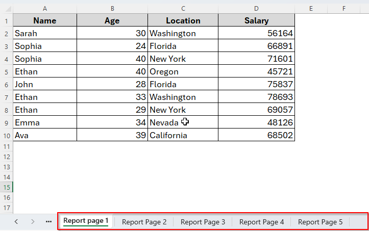
Luckily, we can make headers repeat on every printed page. Let’s see how it works.
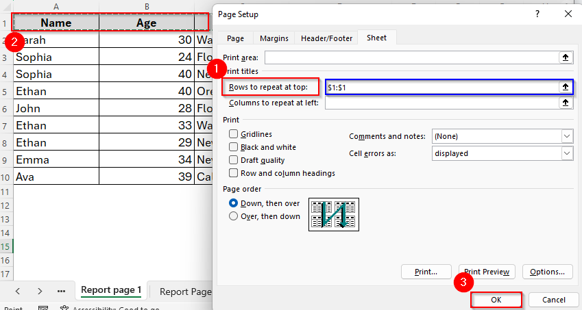
Steps:
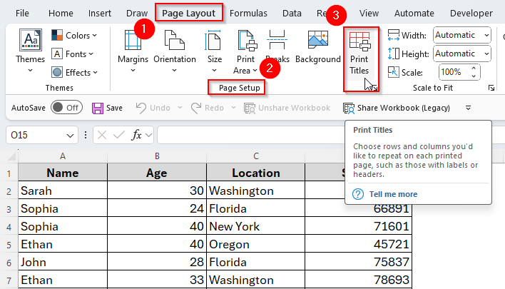
➤ Locate the Page Layout tab.
➤ Choose Print Titles under the Page Setup.
➤ In the rows to repeat at top box, select the row where your headers live (here Row 1).
➤ Hit OK.
Alternative Way to Convert Data to Table for Creating Column Headers
There’s also an alternative method to create Table while adding column headers in excel. This also seems slightly simpler than the previous method we discussed. Personally, I also prefer this method while working with larger worksheets. Below are the steps to follow.
Steps:
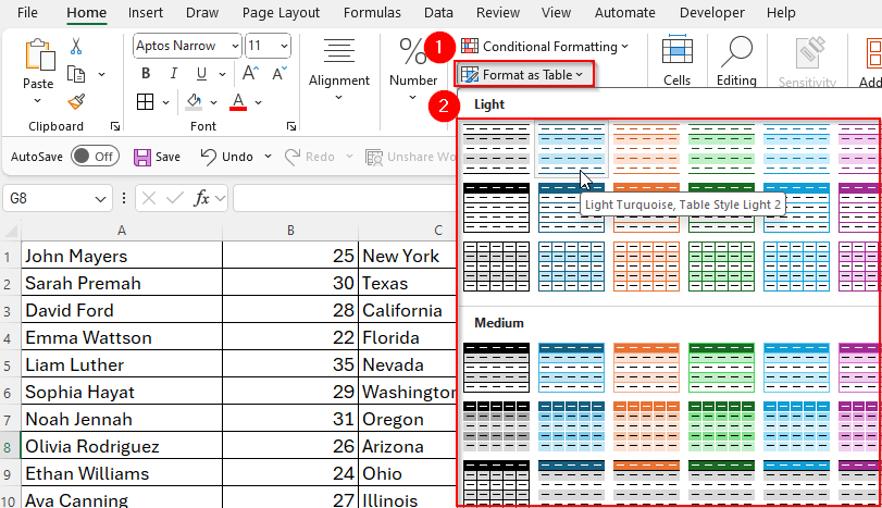
➤ Select Format as Table option from the Ribbon. Here you’ll see various color options. Choose whatever you like.
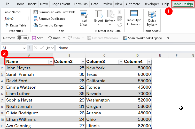
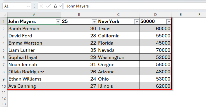
➤ Once you select the color, the table will ultimately be created as in the following image. The first row will work as column headers and you can also edit that as you need.
➤ But if you want to keep the first row intact, and want a completely different row for column headings, then attach a new row before creating the table as we discussed earlier.
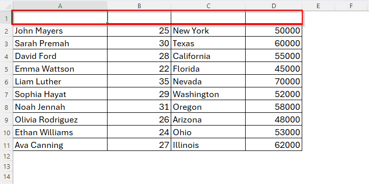
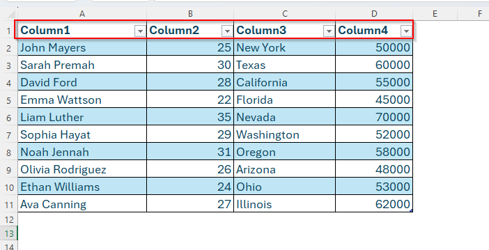
➤ Now if you format the table, it will have a completely new row including multiple column headers as we have Column 1, Column 2, Column 3, and Column 4.
Frequently Asked Questions (FAQs)
Can I make my headers bold or colored?
Yes, definitely. Just select the header cells, then use the Font tools to make them bold, bigger, or colorful.
What if I don’t add headers?
Without headers, it’s hard to know what the data means. Always add them for clarity.
Can I rename a header later?
Yes, just click the header cell and type a new name. You can edit anytime and everytime you want to do it.
Concluding Words
Column headers are definitely very simple, yet they’re one of the most important parts of building a clear, usable Excel sheet. Whether you’re working with a tiny list or a massive dataset, headers act as your compass, keeping everything organized and understandable.
So next time you open Excel, don’t skip this step. Think of headers as your dataset’s storytelling tool. They explain what’s going on without you having to say a word. So, hopefully you find this article helpful.