When you deal with data that repeats often, like product codes, employee IDs, or country names, it can quickly become tiring to type them again and again. It takes extra time, alongside increasing the chance of making mistakes. Instead of typing the same information over and over again, you can store it once in a separate table and have Excel fetch it automatically. It helps maintain your main sheet neat, ensures that the details stay consistent, and makes updates easier. Instead of correcting the same entry across different places, you only need to update it once, and Excel will take care of the rest.
This article will walk you through different ways to create and use a lookup table in Excel. You’ll see both modern and traditional functions, along with a few easy tricks to make your data entry faster and more reliable.
Steps to create a basic lookup table using the XLOOKUP function in Excel:
➤ Create a small table on a separate sheet as your lookup table.
➤ In your main sheet, type this formula to get a matching result:
=XLOOKUP(B2, Lookup!$A$2:$A$11, Lookup!$B$2:$B$10)
➤ This retrieves the matching result from your lookup table from another sheet.
➤ Any changes to the lookup table will update results instantly.
Create a Lookup Table using XLOOKUP Function
XLOOKUP is the modern, flexible lookup function available in Excel 365 and Excel 2021. It replaces VLOOKUP and HLOOKUP, works both vertically and horizontally, and lets you see a custom message if a match is not found.
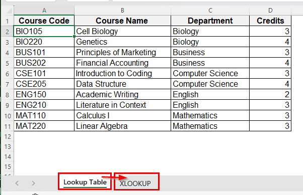
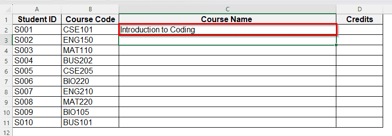
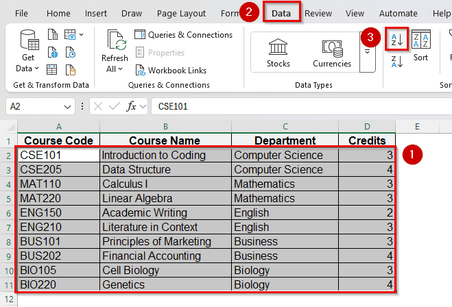
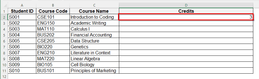
Before applying XLOOKUP, we’ll create a lookup table. This table stores all course information as a list: Course codes, Course names, Departments, and Credits. This sheet acts as the main reference table. The XLOOKUP function is ideal here because it searches for each course code in the lookup table and returns the exact Course Name or Credit linked to it. Any change in the lookup table instantly updates the main table.
Steps:
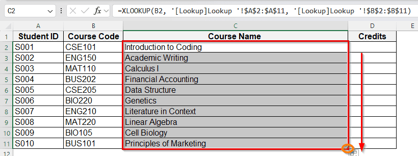
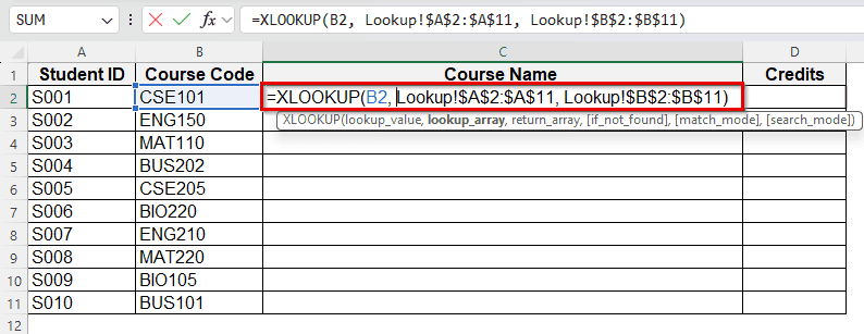
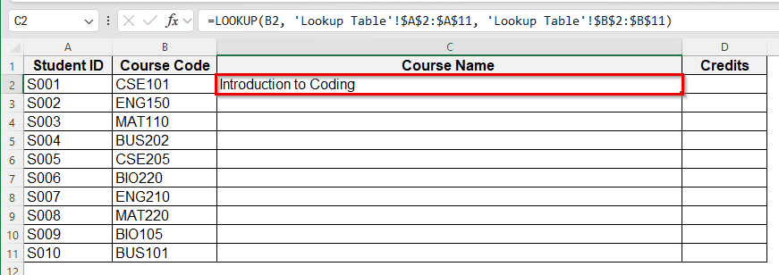
➤ In your main sheet, select a cell, C2, where you want the name to appear using XLOOKUP.
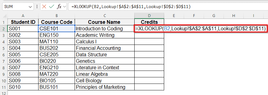
➤ Now type the formula:
=XLOOKUP(B2, Lookup!$A$2:$A$11, Lookup!$B$2:$B$11)
➤ Press Enter > Excel displays the matching description from your lookup table.
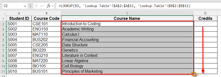
➤ Drag the fill handle down to get results for the rest of the cells in Column C.

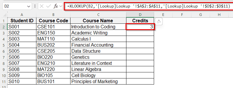
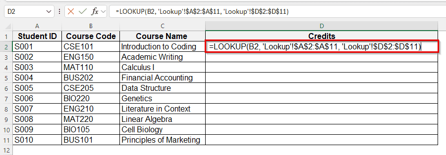
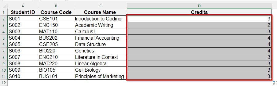
➤ Repeat with Credits column, column D:
=XLOOKUP(B2, Lookup!$A$2:$A$11, Lookup!$D$2:$D$11)
➤ Press Enter, and Excel will display matching results, credit from your lookup table.
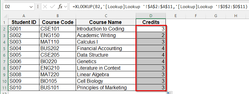
➤ Again, drag the fill handle down, and the rest of the cells will display matching results from the lookup table.
Create a Lookup Table Using VLOOKUP
VLOOKUP has been a standard lookup tool for decades. It searches for a value in the first column of a table and returns a value from a specified column in the same row.
Steps:
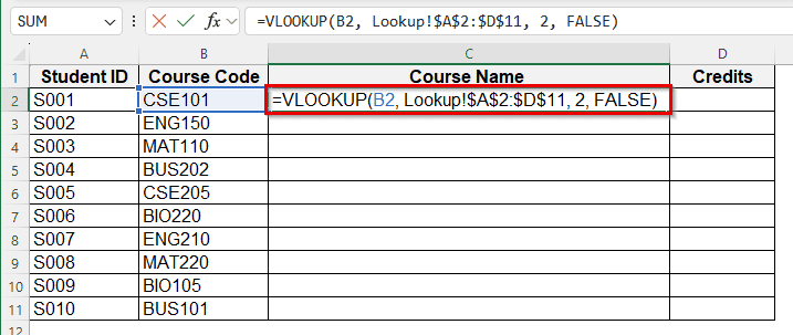
➤ In your main sheet, select a cell C2 where you want the name to appear.
➤ Type the formula:
=VLOOKUP(B2, Lookup!$A$2:$D$11, 2, FALSE)
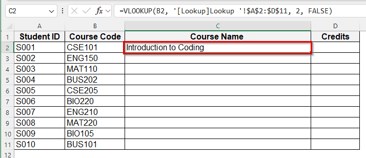
➤ Press Enter for results.
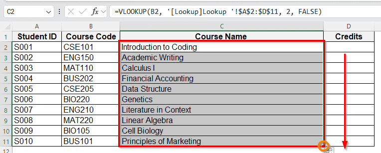
➤ Drag the fill handle down to get results for the rest of the cells in Column C.
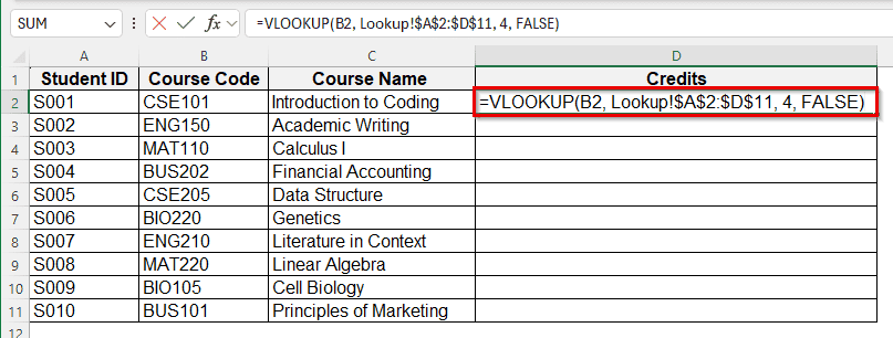
➤ Then repeat with credits column:
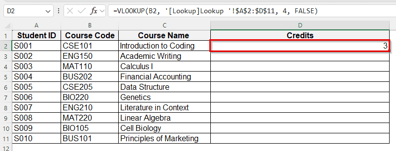
=VLOOKUP(B2, Lookup!$A$2:$D$11, 4, FALSE)
➤ Press Enter, and your desired match will be displayed in cell D2.
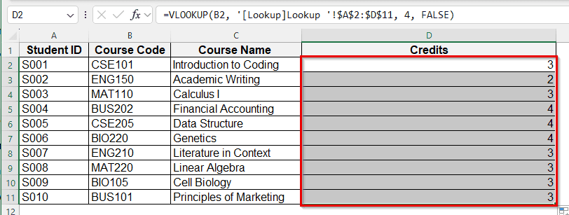
➤ Again, drag the fill handle down, and the rest of the cells will display matching results from the lookup table.
Note:
The “2” and “4” instruct Excel to return data from the second and fourth columns of the lookup table. Here, False is sed to find an exact match. The returned values update automatically in case of any alteration.
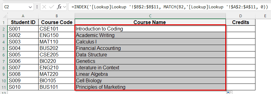
Create a Lookup Table Using INDEX-MATCH Formula
INDEX and MATCH functions together are more flexible than VLOOKUP or HLOOKUP. These functions together allow lookups in any direction and are less affected by inserting or moving columns.
Steps:
➤ In your main sheet, select a cell C2 where you want the result.
➤ Type the formula:
=INDEX(Lookup!$B$2:$B$B11, MATCH(B2, Lookup!$A$2:$A$11, 0))
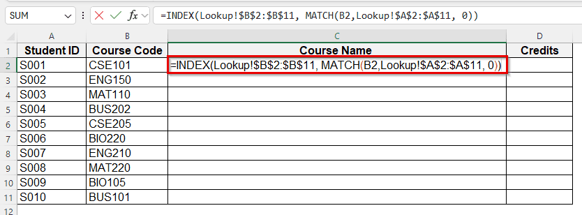
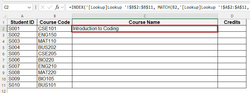
➤ Press Enter for results.
➤ Again, drag the fill handle down to get results for the rest of the cells in column C.
➤ Then repeat with Credits Column:
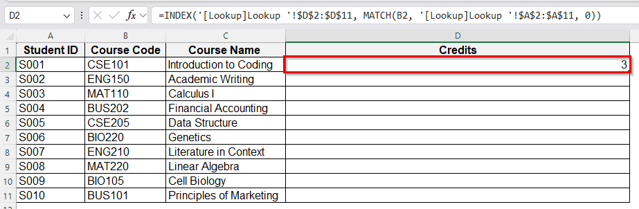
=INDEX(Lookup!$D$2:$D$B11, MATCH(B2, Lookup!$A$2:$A$11, 0))
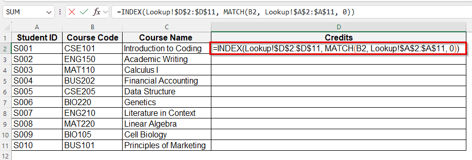
➤ Press Enter, and your desired match will be displayed in cell D2.
➤ Drag the fill handle down to get results for the rest of the cells in Column C.
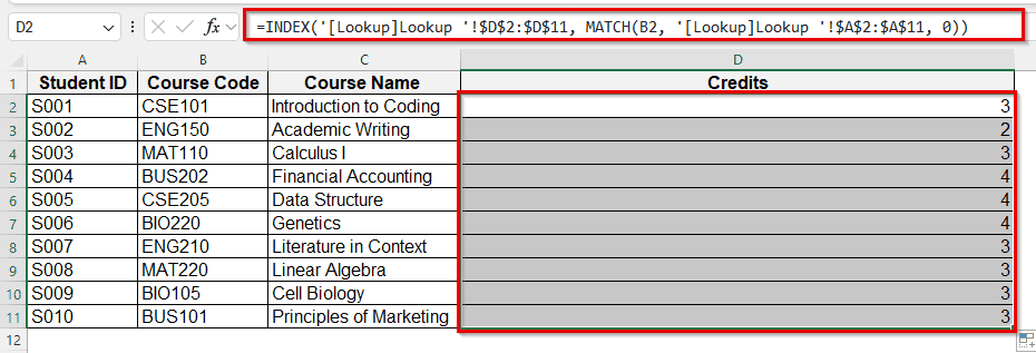
Note:
Match shows the row number when the code is entered, INDEX uses that to return the value from column C. The “0” in MATCH ensures exact matching.
Create a Lookup Table Using LOOKUP Function
LOOKUP function is simpler yet less precise, as it assumes your lookup range is sorted and returns the closest match.
Steps:
➤ Sort your lookup range in an ascending order.
➤ Select the cell, C2 in your main sheet..
➤ Type the formula:
=LOOKUP(B2, Lookup1$A$2:$A$11, Lookup!$B$2:$B$11)
➤ Press Enter and Excel shows the matching results.
Note:
Use in case of sorted data and approximate matches being acceptable.
➤ Drag the fill handle down to get the rest of the matches.
➤ Repeat this with column D.
Drop-Down List for Easy Lookup Selection
Adding a drop-down list helps you choose values instead of typing them, which keeps your entries uniform and saves time. It also reduces small mistakes that can break a lookup. Once added, the list works smoothly with your formulas.
Steps:
➤ Select the cell, C2, where you want the drop-down.
➤ Go to Data > Data Validation > Data Validation.
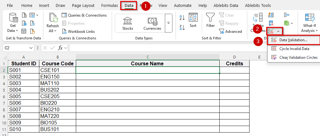
➤ Now you can see an “Allow” box > choose the List option.
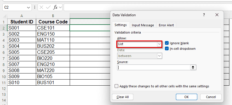
➤ In the “Source” box, select your lookup table sheet and then the range, from B2 to B11.
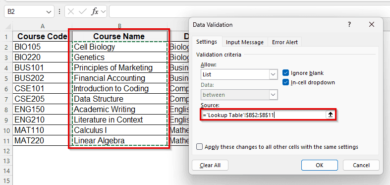
➤ Now click OK and the drop-down will appear
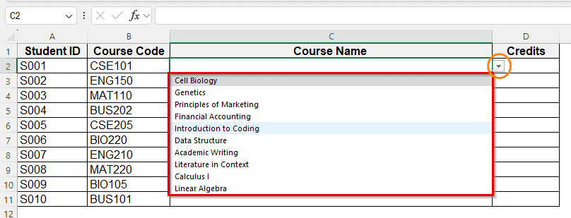
➤ Click the ‘drop-down’ icon to see list of course names.
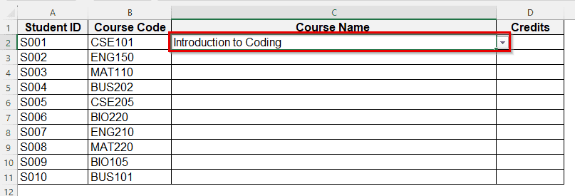
➤ Here is the result.
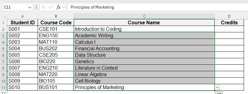
➤ Use the drop-down for other cells in column C.
Frequently Asked Questions
Do I need to keep my lookout table on a separate sheet?
No, but keeping it separate makes it easier to maintain and prevents accidental changes.
What happens if the lookup value is not found?
XLOOKUP displays a custom message. VLOOKUP and others is wrapped in IFERROR to handle missing values.
Can I create a lookup table between two different workbooks?
Yes, but the source workbook must be open unless you use named ranges or Power Query.
Which method is best for a large dataset?
INDEX + MATCH and XLOOKUP are faster and more flexible.
Wrapping Up
Creating a lookup table in Excel saves time and avoids repetitive typing. Whether you choose the modern XLOOKUP, the familiar VLOOKUP or HLOOKUP, or the flexible INDEX and MATCH, the process is straightforward: store reference data once, link it with a formula, and Excel does the work for you. With a drop-down list, the process becomes more efficient and user-friendly. Try different methods and see which fits your data best. Share your feedback with us.