Data cleaning is a critical step in preparing datasets for analysis, reporting, or visualization. In Excel, we need to work with messy entries, duplicate rows, inconsistent formatting, blank cells, or unwanted symbols. Automating these tasks not only saves time but also ensures accuracy and consistency.
To automate data cleaning in Excel, follow these steps:
➤ Load your dataset into Power Query using “From Table/Range”.
➤ Apply transformations like removing blanks, formatting text, and filtering duplicates.
➤ Load the cleaned data into a new worksheet for analysis.
In this article, we will cover 6 methods to automate data cleaning in Excel, including Power Query, Flash Fill, Text to Columns, the SUBSTITUTE function, Find & Replace, and Remove Duplicates.
Using Power Query to Clean Texts and Remove Empty Entries
Power Query is a powerful built-in tool in Excel that we use to automate data cleaning tasks like formatting, removing blanks, and transforming columns. This is necessary when we work with large datasets that require repeated cleaning steps.
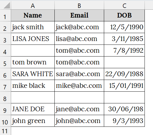
We have a worksheet that contains inconsistent name formatting and blank rows. We will use Power Query to clean the names and remove empty entries, making it ready for analysis or reporting.
Steps:
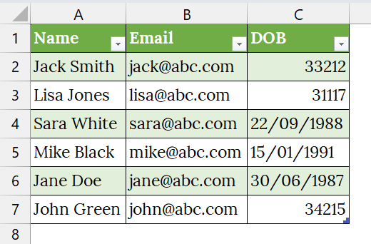
➤ Open your worksheet that contains your data. For example, we have taken a dataset that contains Name in Column A, Email in Column B, and DOB (Date of Birth) in Column C, with inconsistent name formatting and blank rows.
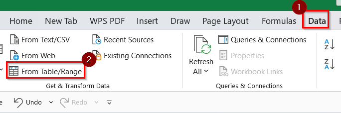
➤ Go to the Data tab → Click From Table/Range.
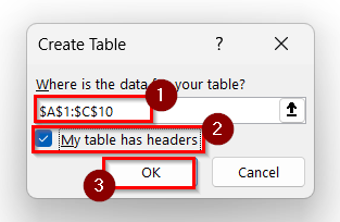
➤ A “Create Table Box” will open. Confirm the range and check “My table has headers”
➤ Click OK.
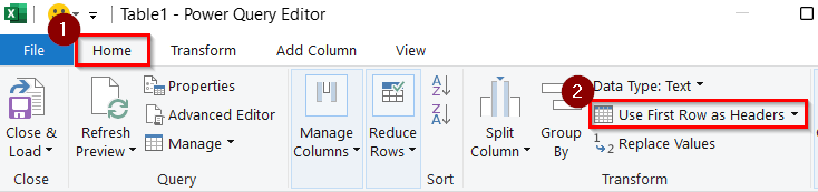
➤ In Power Query Editor, go to the Home tab → Click Use First Row as Headers.
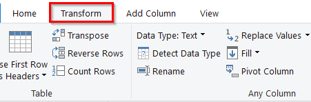
➤ Go to the Transform tab.
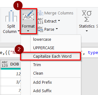
➤ Click Format → Choose Capitalize Each Word.
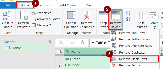
➤ Go to Home tab → Click Remove Rows → Choose Remove Blank Rows.
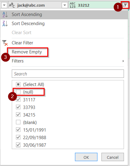
➤ Now, click on the Drop-down arrow of the column that contains blank rows.
➤ Then, uncheck the “Null” → Click Remove Empty.
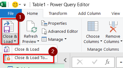
➤ Click Close & Load → Choose Load to New Worksheet.
➤ A dialog box named “Import Data” will open. Choose Table→ New worksheet.
➤ Click OK.
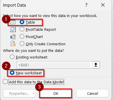
➤ The cleaned data will appear.
Note:
Power Query steps are recorded and reusable. You can refresh the query when new data is added.
Applying the Text to Columns Feature to Split Combined Fields for Cleaner Data
Text to Columns is an Excel feature that splits data from one column into multiple columns based on delimiters such as commas, spaces, or symbols. When we import data from external sources, where various values are packed into one cell, we can use this method too. This method is good for separating names, emails, or addresses into structured columns.
We have a dataset that represents a contact list exported from a CRM system. We will use Text to Columns to split names and emails into separate columns for easier filtering and communication.
Steps:
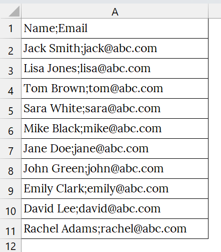
➤ Open your Excel sheet that contains your data. Here, we have taken a dataset that contains Name and Email in Column A, which are separated by delimiters.
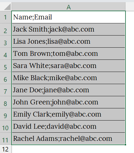
➤ Select the range A1:A11.
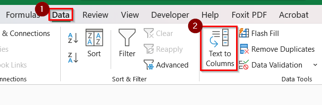
➤ Go to the Data tab → Click Text to Columns.
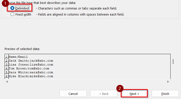
➤ In the Convert Text to Columns Wizard, choose Delimited → Click Next.
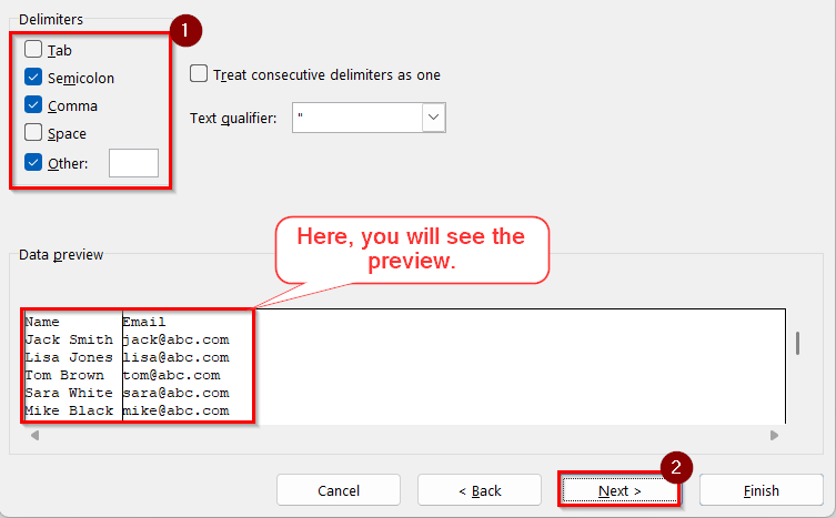
➤ Check Semicolon, Comma, and Others depending on your data. Preview shows how data will be split.
➤ Click Next.
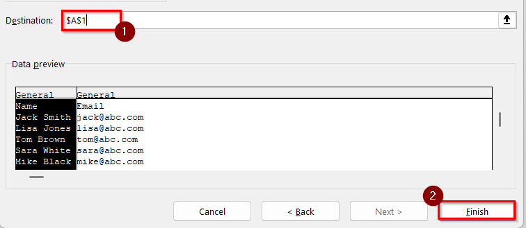
➤ Choose where the split data should appear.
➤ Click Finish.
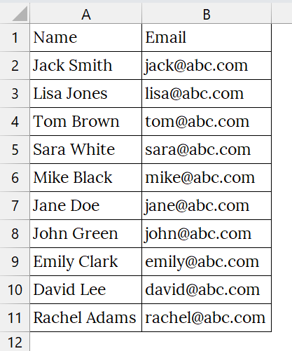
➤ The split and cleaned data will appear.
Note:
If your data uses a unique symbol (e.g., “|”), you can manually enter it as a delimiter.
Automatically Correct Inconsistent Text Formatting in Excel with Flash Fill
Flash Fill is an Excel feature that automatically detects patterns and fills in data based on examples we provide in the first two columns. We can use Flash Fill for cleaning or restructuring data like names, phone numbers, or IDs when the format is inconsistent.
We have a dataset that contains inconsistent employee name formatting in a company. We will use the Flash Fill feature to quickly standardize the names without formulas or manual edits.
Steps:
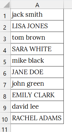
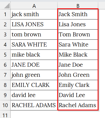
➤ Open your worksheet. Here, we have a worksheet that contains inconsistent name formatting in Column A. For example, “Jack Smith”, “LISA JONES”, etc.
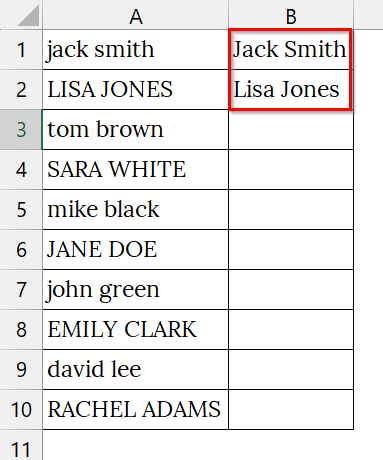
➤ In cell B2 and B3, type the correctly formatted name. For example, Jack Smith and Lisa Jones.
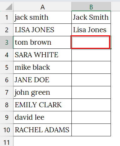
➤ Select cell B3.
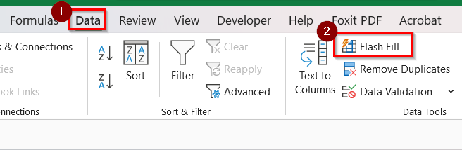
➤ Go to the Data tab → Click Flash Fill.
➤ Excel fills the rest of column B based on your example. Check if all entries are correctly formatted. If needed, manually correct any mismatches and reapply Flash Fill.
Note:
Flash Fill works best when the pattern is clear and consistent.
Using Find & Replace to Remove Unwanted Symbols and Clean Data
Find & Replace is a built-in Excel feature that helps us quickly locate specific characters, words, or patterns and replace them with something else or nothing at all. This is commonly used for removing symbols like “#”, “@”, or “;” from imported data or correcting repeated typos.
We have a dataset corrupted by multiple symbols during import. We will use Find & Replace to clean all entries in seconds, making the data usable for reports or merging.
Steps:
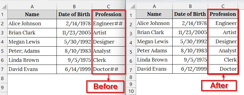
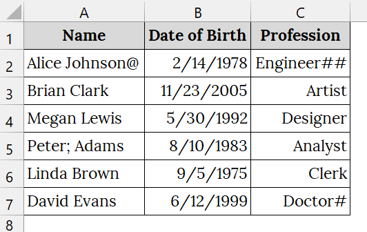
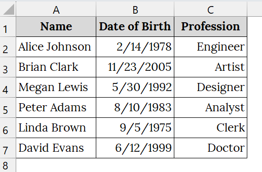
➤ Open your workbook that contains your data. Here, we have taken a dataset that contains Name in Column A, Date of Birth in Column B, and Profession in Column C, which are corrupted by multiple symbols.
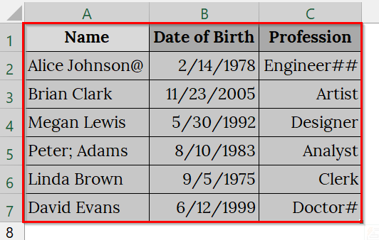
➤ Click and drag to select the whole range.
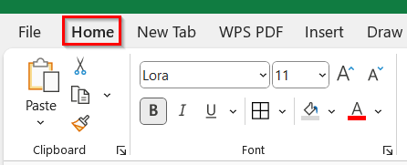
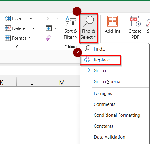
➤ Go to the Home tab.
➤ Click Find & Select → Choose Replace.
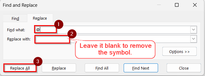
➤ In the Find and Replace dialog:
- In “Find what”, type the symbol (e.g., “@”).
- In “Replace with”, leave it blank to remove the symbol.
- Click Replace All.
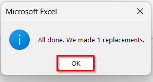
➤ A Microsoft Box will open. Click OK.
➤ The cleaned data will appear.
Automate Data Cleaning by Removing Duplicates in Excel
The Remove Duplicates feature in Excel helps us to eliminate repeated entries from our dataset, ensuring uniqueness in columns like names, IDs, or emails. This method is good for cleaning up contact lists, survey responses, or imported data where duplicates may exist.
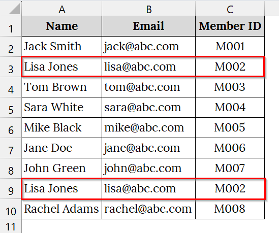
We have an Excel sheet of a membership list with duplicate entries. We will use the Remove Duplicates feature to ensure each member appears only once, making the data ready for reporting or mail merge.
Steps:
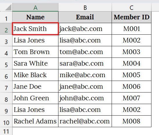
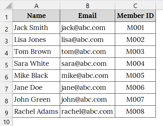
➤ Open your Excel sheet. For example, we have taken a dataset that contains Name in Column A, Email in Column B, and Member ID in Column C with duplicate names.
➤ Click anywhere inside the data range. For example, cell A2.
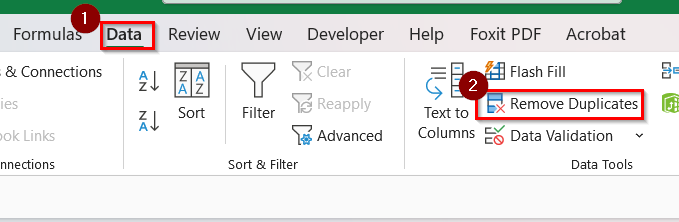
➤ Go to the Data tab → Click Remove Duplicates.
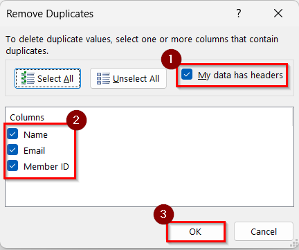
➤ In the dialog box:
- Ensure “My data has headers” is checked.
- Select columns to check for duplicates.
- Click OK.
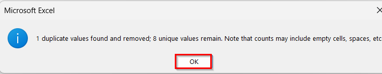
➤ Excel shows how many duplicates were removed and how many unique values remain. Click OK.
➤ The cleaned data will appear.
Note:
➥ If you want to preserve original data, copy it to another sheet before applying this method.
➥ You can apply Remove Duplicates to one or multiple columns depending on your criteria.
Using the SUBSTITUTE Function to Remove Unwanted Characters from Text Data
The SUBSTITUTE function in Excel replaces specific characters or text within a cell. We use it for cleaning up unwanted symbols like “@”, “#”, or “;” from imported data. You should use it when you find that the same unwanted character appears consistently across a column, such as email lists or product codes.
We have a worksheet that contains names corrupted by symbols during import. We will use the SUBSTITUTE function to clean each entry, making it suitable for reporting or merging with other datasets.
Steps:
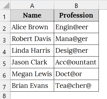
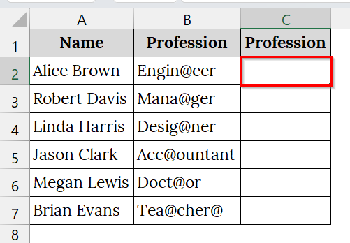
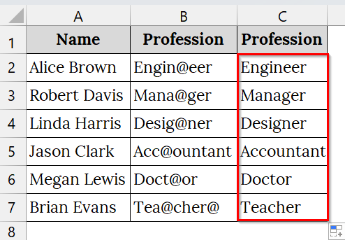
➤ Open your worksheet that contains your data. For example, we have taken a dataset that contains Name in Column A, and Profession in Column B. Here, Column B contains professions with unwanted symbols like Engin@eer, Mana@ger, etc..
➤ Add a new column. For example, Column C.
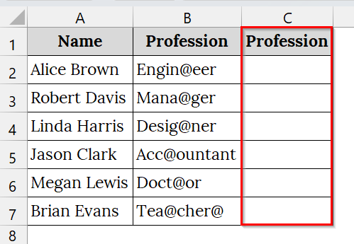
➤ Select cell C2.
➤ In cell C2, enter the formula:
=SUBSTITUTE(B2,"@","")
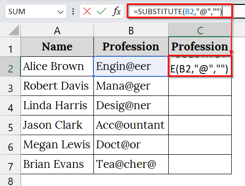
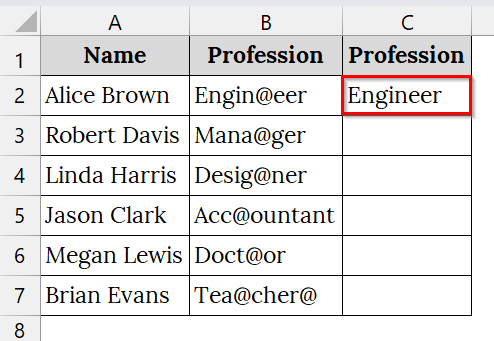
➤ This removes the “@” symbol from the text in C2.
➤ Click and drag the Fill Handle down from C2 to apply the formula to other rows.
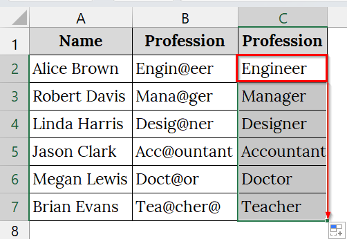
➤ The cleaned data will appear in Column C.
Note:
SUBSTITUTE is case sensitive and only replaces exact matches.
Frequently Asked Questions
Can I automate cleaning for multiple sheets at once?
Yes, using Power Query, you can combine and clean data from multiple sheets or workbooks.
Is Flash Fill dynamic like formulas?
No, Flash Fill is static. For dynamic updates, use formulas like SUBSTITUTE or TEXT functions.
How do I remove symbols like “@” or “#”?
Use the SUBSTITUTE function or Find & Replace to remove unwanted characters.
What if my dates are inconsistent?
Use Format Cells to standardize date formats or Power Query to convert text to a date.
Can I undo automated cleaning steps?
Yes, Power Query maintains a step history that you can edit or remove anytime.
Concluding Words
Automating data cleaning in Excel is no longer a difficult task. With methods like Power Query, Flash Fill, Text to Columns, SUBSTITUTE, Find & Replace, and Remove Duplicates, you can clean large datasets efficiently and accurately. You can download the datasets we have used in this article to practice.