Some Excel users refer to Floating Tables as tables that move freely anywhere on the sheet. However, other users want floating tables that float on the screen as they scroll and change tabs while also moving freely.
While all Excel tables are movable, there aren’t any built-in options in Excel to create a floating table. We can only try a few workarounds to make table data appear across sheets. To simply move a table, the best way is to turn it into a picture.
Steps to freely move an Excel table anywhere in a sheet:
➤ Copy your entire table, including the headers, using the Ctrl + C keyboard shortcut.
➤ Right-click on the cell where you want the new movable table and press the four-sided arrow sign beside the Past Special option.
➤ From the given choices under the Other Paste Options group, select the Picture (U) icon. Excel will turn your table into a movable image. Click on the picture and use the arrow to move the table.

Apart from this method, we’ll cover more ways of creating a floating Excel table using Freeze Pane, Camera Tool, Watch Window, and VBA macro.
Move an Excel Table Using the Four-Sided Arrow on the Table Border
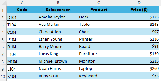
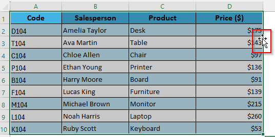
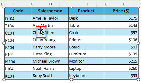
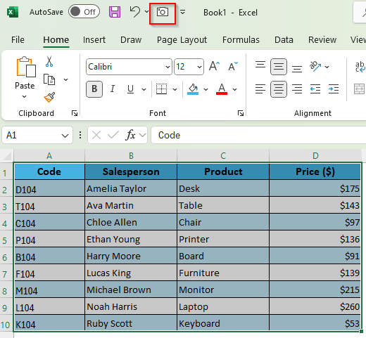
In our sample dataset, we have four columns to represent some product Codes, Salesperson names, Product list, and Prices. We’ll select the range and press Ctrl + T to turn our range into a table.
All Excel tables are movable, so you can place them anywhere in the sheet. However, the arrow you need to use for this isn’t visible, and using it can be tricky. Here’s how to access it.
➤ Select your table and hover the mouse over the border of the table until the cursor becomes a four-sided arrow (move handle).
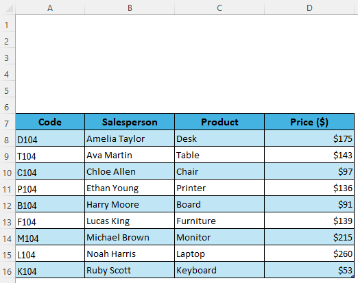
➤ Hold and drag the arrow to move the table to a new location. This way, you can keep the table structure, formatting, and filters intact. We’ve moved our current range from A1:D10 to A7:D16.
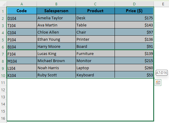
➤ Here’s the moved table:
Turn an Excel Table into a Movable Picture
Although the previous method works, it’s difficult to control the table movement precisely. Therefore, we’ll paste the table as a picture for more flexibility. The only drawback of this method is that it gives you a static picture that doesn’t update when you change your table data.Below are the steps:
➤ Select your table range with the headers. You can click on a header cell and press Ctrl + A to highlight the entire table, including the headers. Press Ctrl + C to copy the table data.
➤ Select the cell where you want to add the new table and right-click on it.
➤ From the menu, click on the Paste Special arrow and choose the Picture (U) option from the Other Paste Options group.
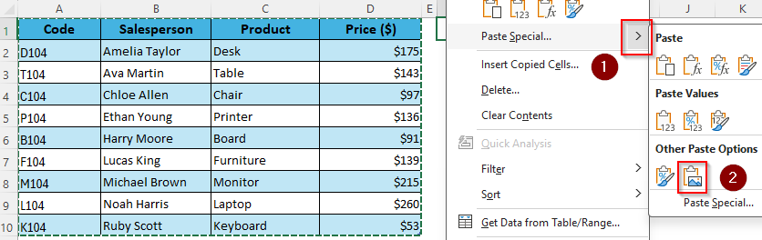
➤ Excel now creates an image version of your table without ruining the table formatting. Click on/hover over anywhere on the image and a small four-sided arrow will appear.
➤ Hold and press on the arrow and place the table anywhere you want within the sheet.
Use the Camera Tool to Make an Excel Table Movable
Similar to the previous method, the Camera Tool allows you to create a live snapshot of a table that floats like an object. The key difference is, when you use the Camera Tool, the picture data updates automatically every time you make any changes in your original table. Let’s get into the details:
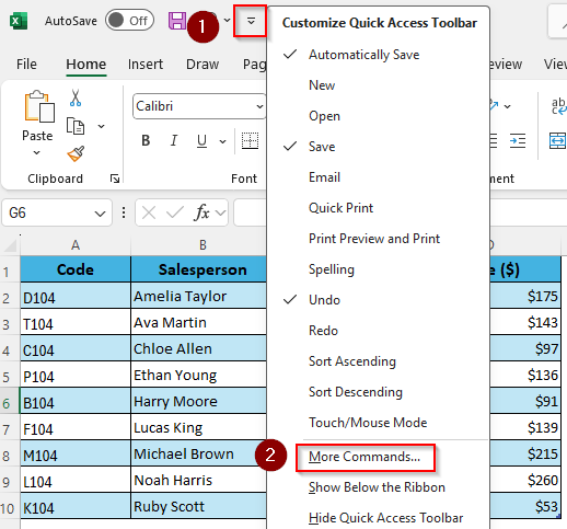
➤ To enable the camera tool, right-click on the Quick Access Toolbar at the top of your screen and select More Commands.
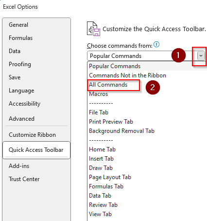
➤ As the Excel Options window opens, select All Commands from the Choose Commands From drop-down.
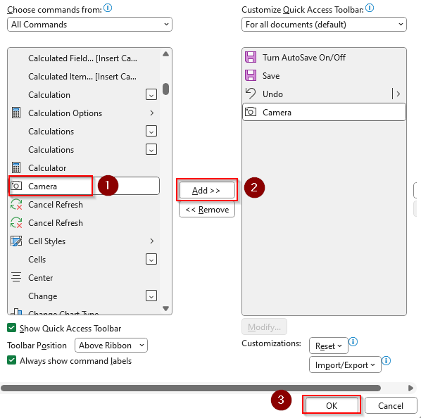
➤ Scroll down and click on Camera. Click on Add >> Ok. Excel will now add Camera (camera icon) to your Quick Access Toolbar.
➤ Select the table range you want to convert into an image and press the Camera icon.
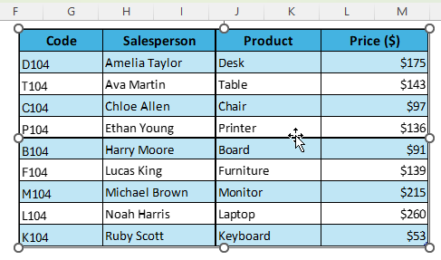
➤ Click anywhere on the sheet to insert a live picture of the table.
➤ Press and drag the move handle to move the snapshot anywhere like a floating table.
Freeze Panes to Keep the Table Fixed While Scrolling
While the above-mentioned methods make a table move freely, the table doesn’t stay fixed as you scroll through the sheet. To lock your table rows and columns so that part of the sheet never scrolls out of view, you need to use the Freeze Panes feature following the steps given below:
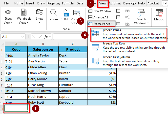
➤ Select the cell below the last row of your table. As our table is in A1:D10, we’re clicking on cell A11.
➤ Go to the View tab and click on the Freeze Panes drop-down from the Window group. Select Freeze Panes from the menu.
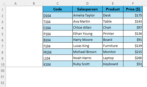
➤ Now, rows 1–10 and columns A–D are locked. You can select the table and move the table anywhere in the sheet, keeping its format intact. When you scroll, the table area stays on screen, and only the rest of the sheet moves. We’ve moved our range with the move handle and the table stays locked in place as we scroll to row 50.
Create a Watch Window with Table Data
If you want your table data to stay fixed as you scroll and change tabs, you can load the table data into the Watch Window. Although it removes the fill color and table style, it’s the only way to keep your table data fixed and visible across sheets. Here’s how:
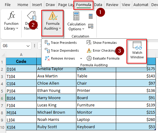
➤ Go to the Formulas tab and click on the Formula Auditing drop-down in the Calculation group. Select Watch Window.
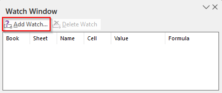
➤ As a floating panel appears, click Add Watch to open a new dialog box.
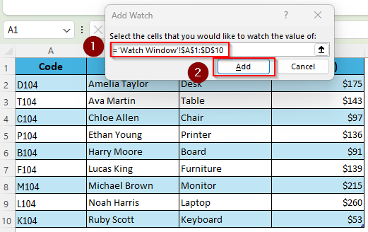
➤ Select the table cell(s) you want to add in the floating window. Use the upward arrow sign to select the range without typing it. Press Add.
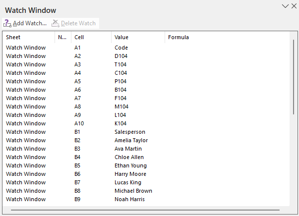
➤ Excel will now load your table data in the floating panel. You can adjust the panel size and expand the columns inside to improve data visibility.
➤ Even if you move to another sheet, the watch window will be docked on top of the sheet.
Create a Floating Table with VBA Macro
In this method, we’ll convert our table into a picture and then use a VBA macro to make a UserForm with that picture so that the table floats as you scroll and change tabs. Here’s how:
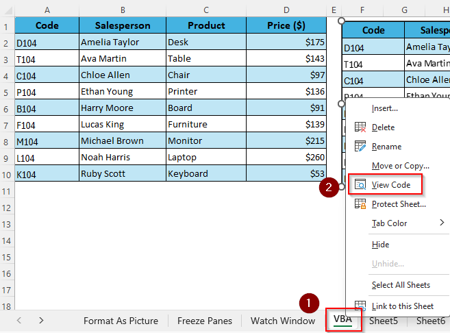
➤ Copy the table, click on the Camera Tool and click on a cell where you want the table image.
➤ Click on the sheet name and select View Code.
➤ In the Module box, paste this code:
Sub ShowFloatingTable()
    FloatingTable.Show vbModeless
End Sub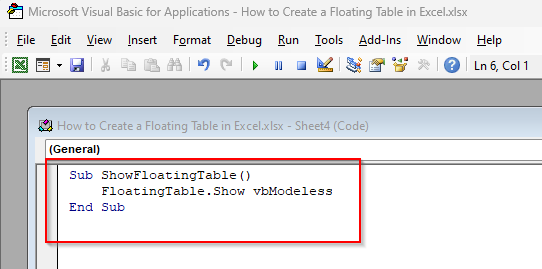
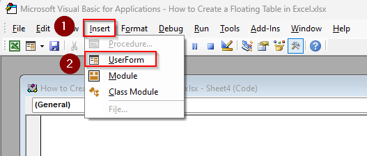
➤ Now, click on the Insert tab and select UserForm.
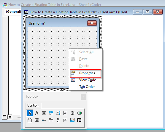
➤ As Excel opens a new UserForm, right-click on it and choose Properties.
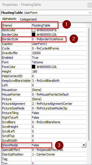
➤ In the Properties box, change the following:
- Name: FloatingTable
- ShowModal: False
- BorderStyle: 0 – fmBorderStyleNone
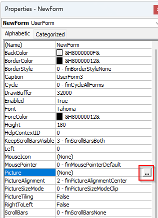
➤ Now, go back to the Excel tab and copy the table image.
➤ Click on the three dots in the Picture box and press Ctrl + V to paste the image in the UserForm box.
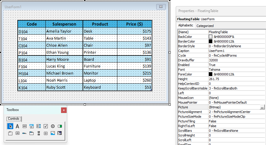
➤ Adjust the size of the UserForm as needed. This will be the size of the floating table that you can’t change later while it’s on the sheet.
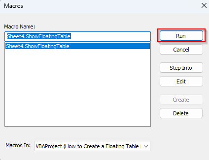
➤ Press F5 or go to the Run tab >> Run Sub/UserForm.
➤ Click on Run if the Macros box pops up.
➤ This will add a floating UserForm to your workbook that stays on top when you scroll or change tabs.
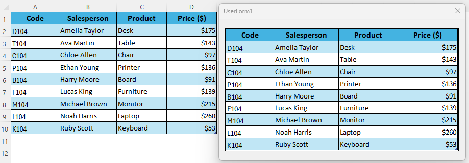
➤ Go back to the Excel tab and scroll down to test the result. Click Ctrl + S to save the code. Click and drag the floating window to move it.
Frequently Asked Questions
How do I get rid of a floating table in Excel?
If the floating table is a converted picture, select the picture and press Delete on your keyboard. For a Watch Window, open the Watch Window, select the watch range, and click Delete Watch. To unfreeze a table, go to the View tab >> Freeze Panes drop-down >> Unfreeze Panes.
How to create a floating comment in Excel?
To create a floating comment, go to the Insert tab and select Text Box. Click inside the box and type your comment. You can place it anywhere and it stays visible while you scroll. If you need it to always stay above the grid, right-click on the box >> Size and Properties >> Properties >> Don’t Move or Size with Cells.
How do I make a floating chart in Excel?
Insert your chart as usual by going to the Insert tab >> Chart. Right-click the chart and select Format Chart Area >> Properties >> Don’t Move or Size with Cells. Now you can drag the chart anywhere and it will behave like a floating object.
Concluding Words
While choosing a method, first decide what output you want. Turn your table into an image to freely move it. Freeze the table rows or the VBA code to keep the table on top while scrolling.
If you want to display the table data in a floating window across sheets, use the given VBA macro or apply the Watch Window trick. In this case, the table data will update automatically when you make any changes in the original table.